Boundary Layer Turbulence#
Ocean-atmosphere exchange occurs via the ocean surface boundary layer (OSBL), a crucial link in the coupling of the air and sea. The nature and intensity of the small scale turbulent motion in this layer strongly affect the fluxes of momentum, heat and gases across the air-sea interface, and deeper into the interior ocean. These small-scale turbulent motions are by computational necessity, parameterized in ocean models with turbulence closure models, in which, the magnitude and distribution of mixing across the OSBL is predicted.
Properties of the OSBL#
in direct contact with the atmosphere: located at the ocean-atmosphere interface
exchange of mass, momentum and energy
varies at short time scales in response to forcing
typically < 100 m deep
lies above the pycnocline
layer that is well-mixed in temperature and salinity is the mixed layer
layer of active turbulence is the mixing-layer
mixing is predominantly driven by shear with episodes of convection
mixing is much larger in the OSBL than deeper below
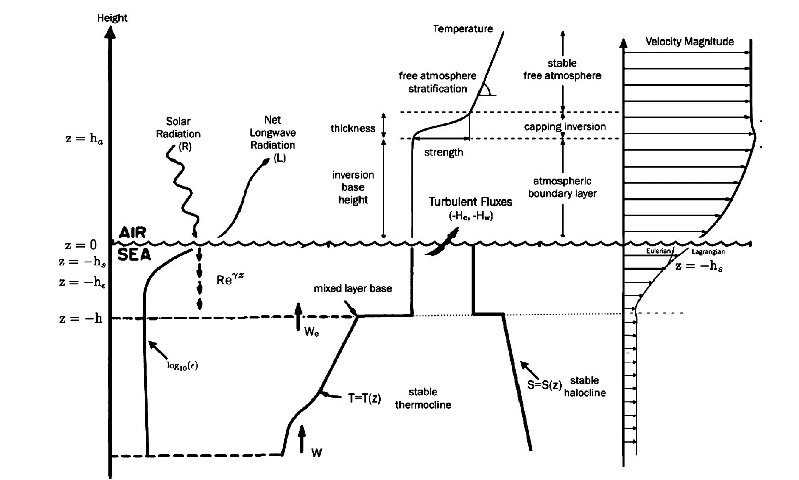
Fig. 11 Schematic of the ocean surface layers, including entrainment velocity, \(w_e\), upwelling, \(w\), temperature, \(T\) salinity, \(S\), turbulent fluxes of thermal energy, \(H_e\) , and freshwater, \(H_w\), dissipation, \(\epsilon\), Stokes depth, \(h_s\), mixing-layer depth, \(h_\epsilon\), and mixed-layer depth, \(h\). Figure 4.2 in Ocean Mixing [FKJQ22].#
Convective Mixing#
Convective mixing is forced by buoyancy forcing (heat and freshwater fluxes). In steady conditions with turbulence dominated by convection, the rate of loss of potential energy in convective plumes, equal to \(B\), provides the energy to balance the dissipation rate, \(\epsilon\), such that:
Under these conditions \(\epsilon\) is approximately constant with depth.
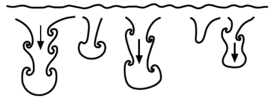
Fig. 12 Convection resulting from cooling at the sea surface (Fig. 3.2, Thorpe, 2007 [Tho07]).#
Wind Stress#
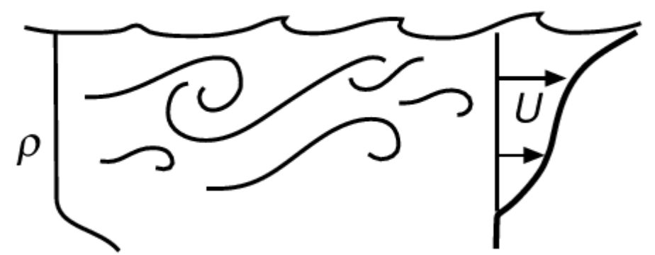
Fig. 13 Turbulence from wind-generated near surface shear flow (Fig. 3.2, Thorpe, 2007 [Tho07]).#
Momentum is transferred into the ocean surface through friction resulting from wind blowing across the rough air-sea interface. When the mean flow and turbulence are steady, such that there is no acceleration, and if we assume a rigid-lid (no surface gravity waves), and if buoyancy flux is negligible, the dissipation rate of turbulence is balanced by the production of kinetic energy of Reynolds stress in the presence of shear (the shear production term), giving:
where \(<u'w'>\) is the Reynolds stress (or momentum flux) approximated by \(\frac{\tau}{\rho_0}\) with \(\tau\) the wind stress, and \(\frac{dU}{dz}\) is the background gradient of horizontal velocity, approximated by the friction velocity \(u_* = \sqrt{\frac{\tau}{\rho_0}}\) and \(z\), the distance from the boundary, such that:
where \(\kappa\) is the von Kármán constant, ~0.41.
Then,
Integrating the shear leads to an equation describing the variation of the mean velocity with distance from the boundary as a log profile, known as the “law of the wall”.
where \(z_0\) is derived as a constant of integration and known as the roughness length scale because it depends on the suze of the boundary roughness. This relationship was first recorded by von Kármán in 1930.
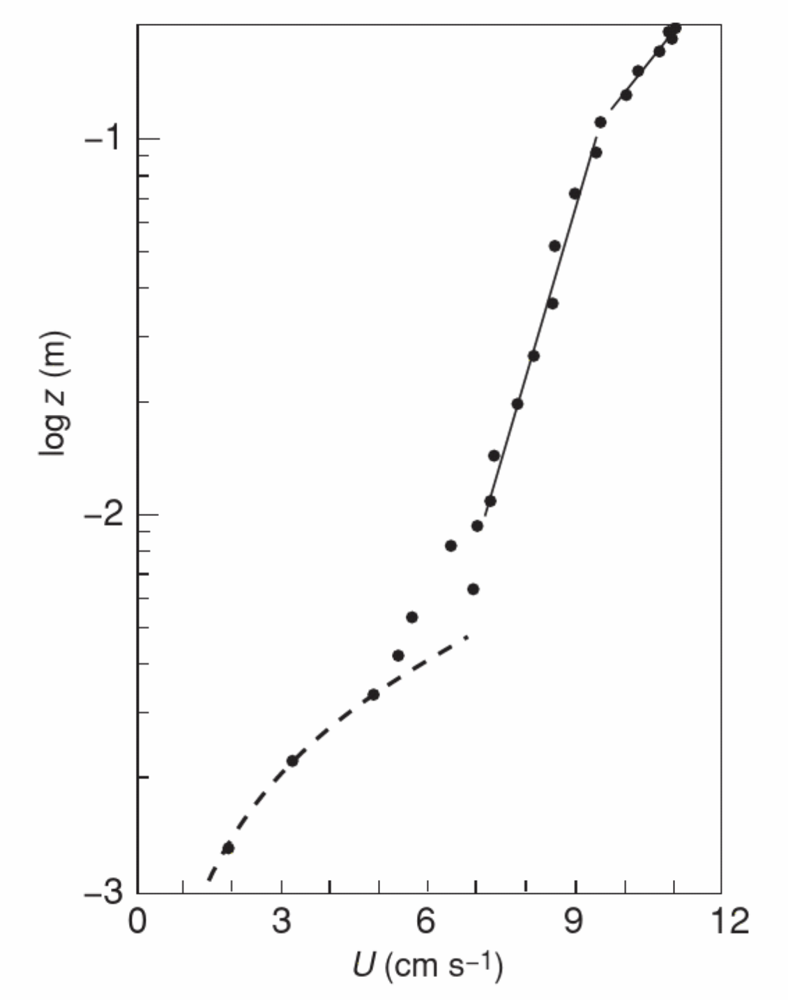
Fig. 14 A logarithmic bottom layer. The mean horizontal flow speed, \(U\), with \(z\), is plotted on a \(log_{10}\) scale, where \(z\) is distance from the seabed. There is a viscous sublayer close to the boundary, below the lower of two layers in which \(U \propto log_{10}z\). Fig. 3.5 in Thorpe 2007 [Tho07].#
Stress and convection: Monin-Obhukov Similarity Theory#
In most geophysical cases, both a buoyancy flux (non-neutral conditions) and stress are actively forcing the surface of the ocean.
Semi-empirical boundary layer similarity theory provides a framework for predicting the vertical structure of mean vertical gradients in the surface layer of wall-bounded turbulent boundary layers given only knowledge of forcing parameters at the wall.
Monin-Obukhov similarity theory (Monin and Obukhov, 1954) states that under horizontally homogeneous and stationary conditions, the only parameters (independent variables) governing the structure of a surface layer are the distance from the boundary, \(z\), the friction velocity, \(u_*=\sqrt{\frac{\tau}{\rho_0}}\) with \(\tau\) the wind stress, and the surface buoyancy flux, \(b^* = B_o/u_*\). The vertical shear and stratification then become functions of one dimensionless group known as the stability parameter, a function of distance from the wall, \(z\), and the Monin-Obukhov length scale, \(L\).
where \(L = \frac{u_*^3}{\kappa B_0}\). The Monin-Obukhov length scale characterizes the balance between shear driven turbulence and buoyancy driven turbulence. Near the boundary, \(z < 0.03|L|\), buoyancy has little effect and the law of the wall is generally valid. In destabilizing conditions, with \(L<0\), mixed conditions in which both shear and buoyancy affect turbulence occur within the range of distances \(0.03|L| < z < |L|\). At distance \(z < 0.3|L|\), buoyancy has a moderate effect, and shear still dominates. At distances \(z < |L|\), buoyancy dominates, driving “free convection”.

Fig. 15 A schematic representation of turbulence and flow near a boundary in different buoyancy regimes. Under convective conditions, horizontal velocity will be reduced compared to neutral and under stabilizing conditions, shear turbulence will be suppressed and horizontal velocities will be enhanced (e.g. diurnal jet). (Fig 3.6, Thorpe 2007).#
When convective conditions occur, convection overturning cells mix out vertical shear, reducing shear production relative to LOW. Under stabilising buoyancy forcing, vertical shear is enhanced, increasing shear production relative to LOW. This scaling of vertical shear is related to buoyancy forcing through the stability parameter, \(\zeta\), related to the Monin-Obukhov lengthscale.
The effects of buoyancy forcing on the canonical “law of the wall” was shown empirically in the Kansas experiments over wheat fields in 1971 [BWIB71] by measuring wind speeds with anemometors and the fluctuating wind components with sonic anemometors.
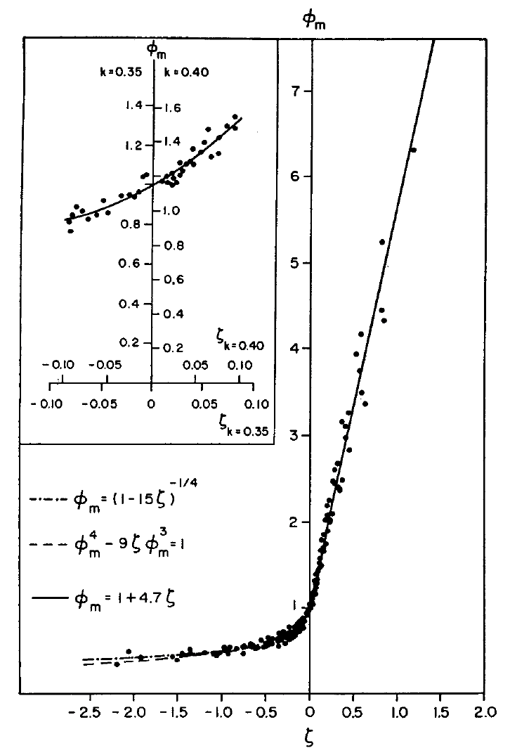
Fig. 16 Comparison of dimensionless wind shear observations taken during the Kansas Experiment (Fig 1., Businger et al., 1971)#
In the figure above, negative \(\zeta\) represents destabilizing conditions, while positive \(\zeta\) represents stabilising conditions. At \(\zeta=0\), forcing is neutral and the non-dimensional vertical shear \(\phi=1\), where \(\phi=\frac{du}{dz} \frac{\kappa z}{u_*}\). Under destabilising forcing, \(\phi\) is less than 1, reducing the LOW predicted shear and under stabilising forcing, \(\phi\) is greater than 1, increasing shear compared to LOW.
In this way, the “law-of-the-wall” approximation for dissipation can be modified to a function of both friction velocity, \(u_*\) and buoyancy, \(B_0\).
where \(\mathrm{A}\) and \(\mathrm{B}\) are empirically defined constants (e.g. Lombardo and Gregg, 1989) [LG89].
Wave-driven mixing processes#
There are three main sources of wave-driven turbulence: Breaking waves, Stokes drift shear and Langmuir turbulence.
Breaking Waves
When waves reach a critical steepness they break, injecting TKE in the wave breaking layer of the OSBL. The depth to which wave-breaking enhanced dissipation impacts the OSBL is a function of the significant wave height.
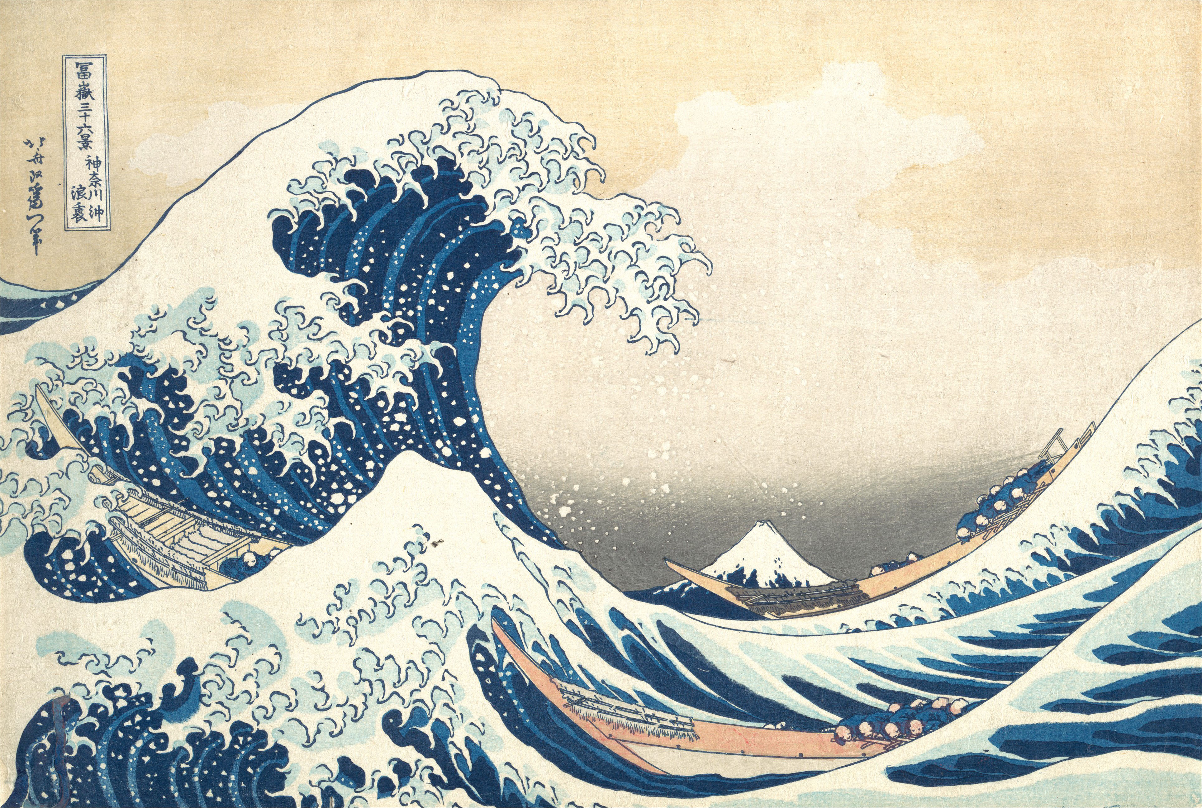
Fig. 17 The Great Wave off Kanagawa by Katsushika Hokusai. 1931. Source: Wikipedia.#
Stokes Drift
When winds blow over a fluid, waves are formed. Surface gravity waves are simply defined as orbital waves that decay exponentially with depth, but they are not perfectly orbital: moving slightly faster at the crest and slower at the troughs due to the return flow. This results in a small but not insignificant current confined to the wave impacted layer of the OSBL. The shear associated with Stokes drift adds an additional source of turbulence.
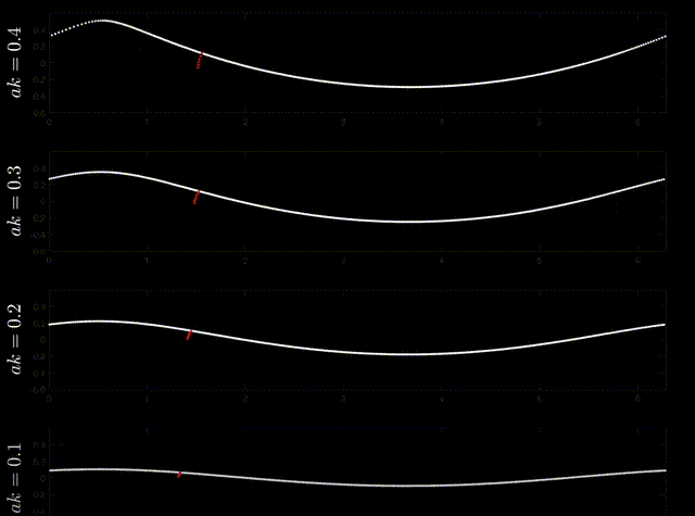
Fig. 18 Particle trajectories (red) of permanent progressive irrotational inviscid deep-water surface gravity (ie Stokes) waves. Source: Nick Pizzo, https://youtu.be/htClUyNKRrU?si=5ZcLl_hCiWZEVtsv.#
Langmuir Turbulence
Dr. Irving Langmuir noted large quantities of floating seaweed arranged in parallel lines with spacing between 100 - 200 m (Langmuir, 1938). THe streaks were parallel to the wind direction and appeared to follow the ambient wind direction. Following this observation, Langmuir ran an experiment in a lake to test the hypothesis that these streaks were a result of overturning cells linked to wind and wave forcing. Today known as Langmuir cells. Langmuir cells form as a result of the interaction between the background vertical vorticity forced by winds and the Stokes drift current which converts vertical vorticity to the horizontal vorticity. It has become broadly accepted that wave driven Langmuir cells are ubiquitous in the ocean and play an important role in the turbulent flux of matter and momentum. The intensity of Langmuir turbulence is described by the turbulent Langmuir number, \(La_t = \sqrt{\frac{u_*}{U_s}}\), where \(U_s\) is the Stokes drift.
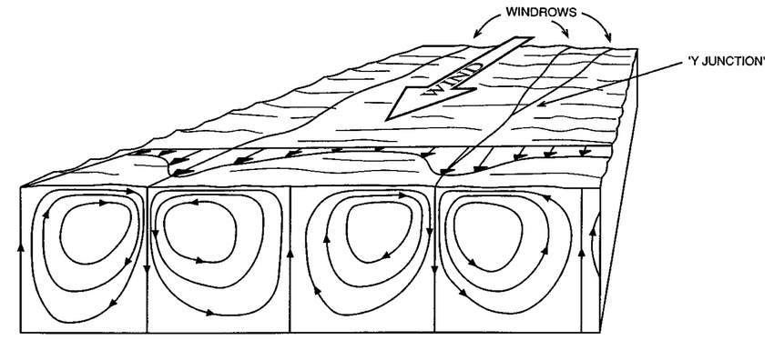
Fig. 19 Langmuir circulation. A sketch of the circulation pattern. Windrows composed of floating materal or foam form as a consequence of convergent motion at the water surface (Fig 3.12, Thorpe 2007).#