Predicting turbulent flows#
Flow in the ocean can be quantitatively described and forecast using a basic set of equations:
The Continuity Equation:
\(\nabla \cdot \mathbf{u} = \frac{\partial u}{\partial x} + \frac{\partial v}{\partial y} + \frac{\partial w}{\partial z}\)The Momentum Equations (Navier-Stokes with rotation)
The Equation of State:
\(\rho = \rho(\mathrm{T}, \mathrm{S}, \mathrm{p})\)The Conservation of scalar properties (e.g., evolution of temperature and salinity)
The Turbulent Kinetic Energy (TKE) Equation:
\(\frac{\partial{TKE}}{\partial t} = \mathrm{Production} + \mathrm{Buoyancy} + \mathrm{Transport} - \varepsilon\)
Here, we focus on understanding and observing the turbulent terms of the momentum equation and the TKE equation.
We have seen that the ocean is a turbulent system that exhibits a wide range of scales.
Solving for all scales is computationally not feasible.
We use Reynolds averaging as a framework to separate the mean and turbulent components of the flow, resulting in a tractable set of equations for large-scale ocean dynamics, and a turbulent part which can be parameterized.
Reynolds Decomposition and Averaging#
To separate the turbulent part from the mean part of the flow, we apply Reynolds decomposition.
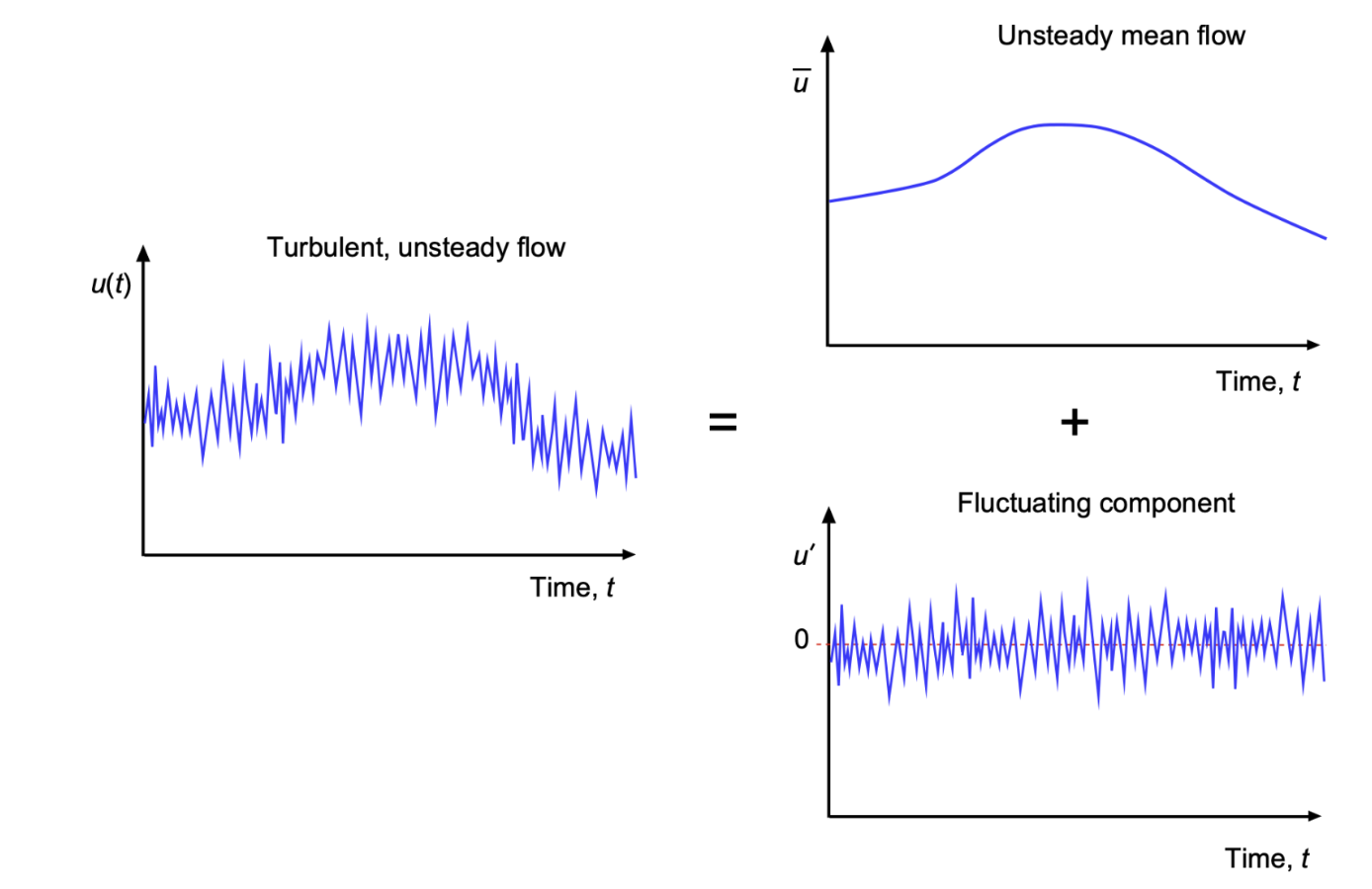
Fig. 5 Reynolds decomposition splits the turbulent flow properties into a statistical mean and a statistically fluctuating part. Source: Embry-Riddle Aeronautical University#
Reynolds Decomposition#
Reynolds decomposition separates the flow variables into a mean component and a fluctuating (turbulent) component:
where:
\( \overline{\mathbf{u}} \) is the mean velocity.
\( \mathbf{u'} \) is the turbulent perturbation.
Similarly, the pressure field is decomposed as:
Reynolds Averaging Rules#
Applying Reynolds averaging, we use the following properties:
The mean of the fluctuation is zero:
\[ \overline{\mathbf{u'}} = 0 \]The mean of a product of a mean quantity and a fluctuating quantity is zero:
\[ \overline{a b'} = \overline{a} \overline{b'} = \overline{a} \cdot 0 = 0 \]\[ \overline{b a'} = \overline{b} \overline{a'} = \overline{b} \cdot 0 = 0 \]The mean of nonlinear terms is not necessarily zero:
\[ \overline{\mathbf{u' v'}} \neq 0 \]For example:
\[ \overline{a'^2}, \quad \overline{a' b'^2}, \quad \overline{a'^2 b'^2}, \quad \overline{a' b'} \neq 0 \]Linearity of averaging:
\[ \overline{a+b} = \overline{a} + \overline{b} \]\[ \overline{a b} = \overline{a} \cdot \overline{b} + \overline{a' b'} \]Double averaging:
\[ \overline{\overline{a} a'} = \overline{\overline{a}} + \overline{a'} = \overline{a} + \overline{a'} = \overline{a} \]
Derivation of the Reynolds-Averaged Momentum Equation#
2. Expanding and Applying Reynolds Averaging#
Taking the Reynolds average and canceling zero terms:
4. Importance of the Turbulent Momentum Flux Term#
The term \( -\overline{\mathbf{u'} \cdot \nabla \mathbf{u'}} \) represents the turbulent momentum flux (Reynolds stress).
This term must be parameterized using a turbulence closure model because solving for \( \mathbf{u'} \) introduces additional unknowns, leading to closure issues.
This formulation is fundamental in turbulent flow modeling, including Large Eddy Simulations (LES) and Reynolds-Averaged Navier-Stokes (RANS) models.
The Turbulence Kinetic Energy (TKE) Equation#
TKE is a direct measure of turbulence in a flow and is one of the most important variables in oceanography. The TKE budget equation provides insights into the physical processes generating and dissipating turbulence. It is directly related to the turbulent fluxes of momentum derived earlier.
Derivation of the TKE Equation#
Turbulent Kinetic Energy (TKE) per unit mass is defined as:
To derive the TKE equation, multiply the fluctuating Navier-Stokes equation by \( u'_i \) and take the Reynolds average. After considerable manipulation the TKE equation for horizontally homogeneous flow emerges.
Here we take cartesian coordinates E.g: \(u_i = u_1 + u_2 + u_3 = u + v + w\)
Solve for z-direction: \(i=1,j=3: u_iu_j = u,w, x_j=z\). Note buoyancy only acts in the z-direction.
Each term simplifies as follows by applying the product rule where applicable:
Rate of change of TKE:
\[ u'_i \frac{\partial u'_i}{\partial t} \]Apply the product rule:
\[ \frac{\partial}{\partial t}(u'_iu'_i) = u'_i \frac{\partial u'_i}{\partial t} + u'_i \frac{\partial u'_i}{\partial t} \]\[ \frac{\partial}{\partial t}(u'_iu'_i) = 2u'_i \frac{\partial u'_i}{\partial t} \]Simplify and take the Reynolds average:
\[ \frac{\partial}{\partial t}(\frac{1}{2}\overline{(u'_iu'_i)}) = \overline{u'_i} \overline{\frac{\partial u'_i}{\partial t}}, \]which is the time rate of change of TKE, \(e\).
thus,
\[ \overline{ u'_i \frac{\partial u'_i}{\partial t} } = \frac{\partial e}{\partial t}. \]Mean flow advection:
\[ u'_i \overline{u}_j \frac{\partial u'_i}{\partial x_j} \]Take \(\overline{u}_j\) out because it is a mean quantity, apply the product rule to \(u'_i \frac{\partial u'_i}{\partial x_j}\), and Reynolds average:
\[ \overline{u}_j \frac{\partial}{\partial x_j}(\frac{1}{2}u'_iu'_i) = \overline{u}_j \frac{\partial e}{\partial x_j} \]Shear production:
\[ u'_i u'_j \frac{\partial \overline{u}_i}{\partial x_j} \]Apply the product rule to give (by applying the product rule twice to the second term):
\[ \frac{\partial}{\partial x_j}(u'_iu'_j\overline{u_i}) - \frac{\partial}{\partial x_j}(u'_iu'_j\overline{u_i}) - u'_i u'_j \frac{\partial \overline{u}_i}{\partial x_j} = u'_i u'_j \frac{\partial \overline{u}_i}{\partial x_j} \]Simplify and take the Reynolds average:
\[ \overline{u'_i u'_j \frac{\partial \overline{u}_i}{\partial x_j} } = -\overline{ u'_i u'_j } \frac{\partial \overline{u}_i}{\partial x_j}. \]Turbulent transport:
\[ u'_i u'_j \frac{\partial u'_i}{\partial x_j} \]Apply the product rule:
\[ \frac{\partial}{\partial x_j}(u'_iu'_ju'_i) = u'_i u'_j \frac{\partial u'_i}{\partial x_j} + u'_i\frac{\partial u'_iu'_j}{\partial x_j} \]Apply the product rule again to the second term on the RHS:
\[ u'_i\frac{\partial (u'_iu'_j)}{\partial x_j} = u'_i\frac{\partial u'_j}{\partial x_j} + u'_j\frac{\partial u'_i}{\partial x_j} \]Because of incompressibility the second term on the RHS cancels, \(\frac{\partial u_x}{\partial x} = 0\)
Substitute back in:
\[ \frac{\partial}{\partial x_j}(u'_iu'_ju'_i) = u'_i u'_j \frac{\partial u'_i}{\partial x_j} + u'_j [u'_i \frac{\partial u'_j}{\partial x_j}] = 2u'_i u'_j \frac{\partial u'_i}{\partial x_j} \]Divide by 2:
\[ \frac{\partial}{\partial x_j}(\frac{1}{2}u'_iu'_ju'_i) = u'_i u'_j \frac{\partial u'_i}{\partial x_j} \]Reynolds average:
\[ \frac{\partial}{\partial x_j}(\frac{1}{2}\overline{u'_iu'_ju'_i}) = \overline{u'_i u'_j \frac{\partial u'_i}{\partial x_j}} \]Pressure transport and strain terms:
\[ -\frac{1}{\rho_0} u'_i \frac{\partial p'}{\partial x_i} \]Apply the product rule and simplify:
\[ -\frac{1}{\rho_0} \frac{\partial}{\partial x_i}(u'_ip') = -\frac{1}{\rho_0} u'_i \frac{\partial p'}{\partial x_i} - \frac{1}{\rho_0} p' \frac{\partial u'_i}{\partial x_i} \]Thus, taking the Reynolds average:
\[ \frac{1}{\rho_0} \overline{u'_i \frac{\partial p'}{\partial x_i}} = \frac{1}{\rho_0} \overline{\frac{\partial}{\partial x_i}(u'_ip')} - \frac{1}{\rho_0} \overline{p'} \overline{\frac{\partial u'_i}{\partial x_i}}, \]where
\(\frac{1}{\rho_0} \frac{\partial}{\partial x_i}(\overline{u'_ip'})\) is the pressure transport term
and
\(\frac{1}{\rho_0} \overline{p'} \frac{\partial \overline{u'_i}}{\partial x_i}\) is the pressure strain term.
Buoyancy production:
The buoyancy production term remains as is:
\[ \overline{ u'_j b' }. \]Viscous diffusion and dissipation:
\[ \nu \overline{ u'_i \frac{\partial^2 u'_i}{\partial x_j \partial x_j} } \]Apply the product rule, using \(a=u'_i\) and \(b=\frac{\partial u'_i}{\partial x_j}\)
\[ \frac{\partial }{\partial x_j}(u'_i\frac{\partial u'_i}{\partial x_j}) = u'_i \frac{\partial^2 u'_i}{\partial x_j \partial x_j} + \frac{\partial u'_i}{\partial x_j}\frac{\partial u'_i}{\partial x_j} \]Rearrange, mulitply back in \(\nu\) and Reynolds average:
\[ \nu \overline{u'_i \frac{\partial^2 u'_i}{\partial x_j \partial x_j}} =\nu \overline{\frac{\partial }{\partial x_j}(u'_i\frac{\partial u'_i}{\partial x_j})} - \nu \overline{\frac{\partial u'_i}{\partial x_j}\frac{\partial u'_i}{\partial x_j}} \]where
\(\nu \overline{\frac{\partial }{\partial x_j}(u'_i\frac{\partial u'_i}{\partial x_j})}\) is the transport of turbulence due to molecular viscosity
and
\(\nu \overline{\frac{\partial u'_i}{\partial x_j}\frac{\partial u'_i}{\partial x_j}}\) is the dissipation rate of turbulence kinetic energy.
Thus, gathering all the transport terms together, the final TKE equation is:
where:
\(\frac{\partial e}{\partial t}\) is the local time rate of change of TKE
\(\overline{u}_j \frac{\partial e}{\partial x_j}\) is the advection of TKE by the mean flow
\(\frac{\partial}{\partial x_j} \left( \frac{1}{2} \overline{ u'_i u'_i u'_j } + \frac{\overline{ u'_j p' }}{\rho_0} - \nu \frac{\partial e}{\partial x_j} \right)\) is the divergence of turbulent transport: turbulent transport of TKE, the resdistribution of turbulence by pressure fluctuations and the transport of TKE due to molecular viscosity.
\(-\overline{ u'_i u'_j } \frac{\partial \overline{u}_i}{\partial x_j}\) is the shear production of TKE/ generation of TKE from the mean flow
\( \overline{ u'_j b' }\) is the buoyancy production or consumption. It can both generate turbulence or suppress turbulence.
\(\varepsilon\) is the dissipation rate of turbulence kinetic energy. Dissipation of TKE can be measured.
The following figure shows the steady state TKE budget for convective and stabilising cases in the ocean surface boundary layer.
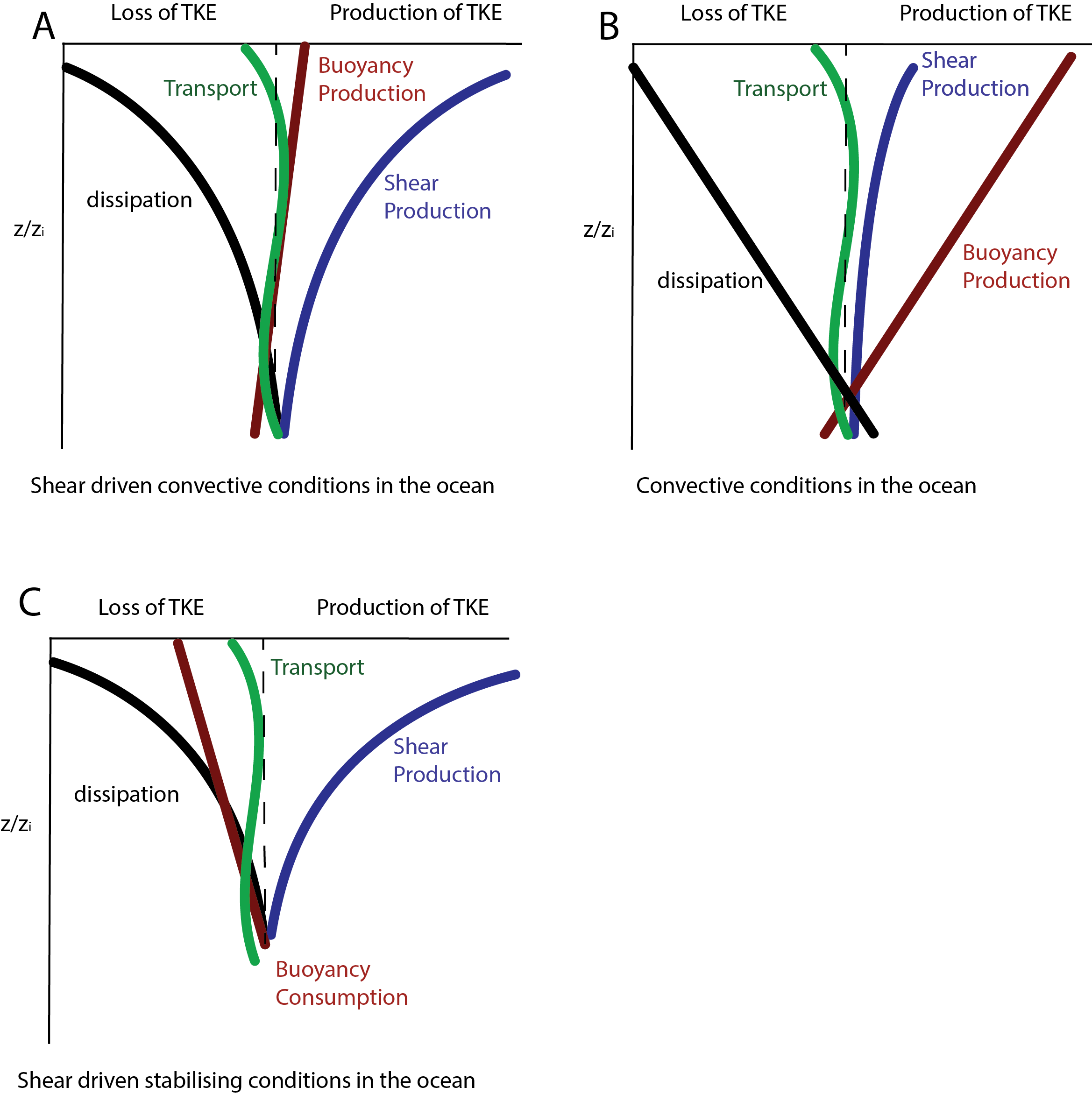
Fig. 6 Schematic of the steady state TKE budget. a) Shear driven convection, b) Convective conditions and c) Stabilising conditions.#