Observing turbulence#
In the lab#
In 1883, Osborn Reynolds described an experiment on the transition between laminar and turbulent flow in a tube. He discovered that the flow resistance was propotional to the flow velocity for small velocities, and proportional to the square of the flow velocity, \(V\), if a certain threshold was exceeded. He found that this critical velocity depended on the diameter, \(D\), of the tube and the molecular viscosity, \(\nu\), of the water. He further notices by visual inspection of streaks of colored water that, at this critical velocity, a transition from direct (straight, laminar) to sinuous (turbulent) motion took place.
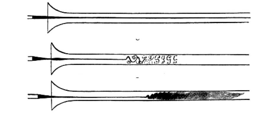
Fig. 7 Osborn Reynold’s experiment. laminar (top panel), transitional flow (middle panel), and fully turbulent flow (bottom panel). The current flows from left to right through a glass tube, with some fluid marked by streaks of colored water.#
Reynolds found in his tube experiments that the non-dimensional number:
named, the Reynolds number. For \(\mathrm{Re}\) smaller than 1900 he found laminar flow, whereas for \(\mathrm{Re}\) larger than 2000, the flow shoed a transition to irregular turbulent motions. The Reynolds number describes the ratio of turbulent diffusivity to molecular diffusivity.
The Richardson number, \(\frac{N^2}{S^2}\), the ratio of background vertical stratification to background vertical shear, quantifies the capacity of a flow to overcome buoyancy suppression and turbulent eddies to form. Typically, a water parcel with a Richardson number of less than 0.25 will have the potential to develop turbulent overturns.
One can use the Buoyancy Reynolds number to quantify turbulence intensity (energetic capacity of a stratified flow to develop overturns) given knowledge of the turbulence dissipation rate and vertical stratification, where \(Re_b = \frac{\varepsilon}{\nu N^2}\). Typically, \(Re_b \leq 20\) is laminar flow, \(Re_b \geq 200\) is turbulent.
The Reynolds number also describes the ratio of small to large structures. Recall da Vinci’s sketch. Highly turbulent fluids will have a large Reynolds number because the number of small structures will be much greater than the number of large structures.
In the ocean#
Turbulent mixing can be observed through examining the small-scale velocity structure of flow in the ocean. Small-scale velocity fluctuations can be measured by microstructure profilers that use an airfoil-shaped shear probes that senses transverse velocity fluctuations caused by turbulent eddies as the profiler moves through the fluid.

Fig. 8 Schematic of an air-foil shear probe. Source: RSI Technical Note 028#
On the scales of meters, the velocity structure is spikey - indicating intense small-scale turbulence. However, on the scale of a few centimeters, the structure is smooth. This is the scale at which the irreversible conversion of TKE into internal energy (heat) by viscous effects takes place. Turbulence creates small-scale gradients that are strong enough to be directly affected by molecular smoothing. The same mechanism can be observed in scaler fluctuations (e.g. gradients of temperature).
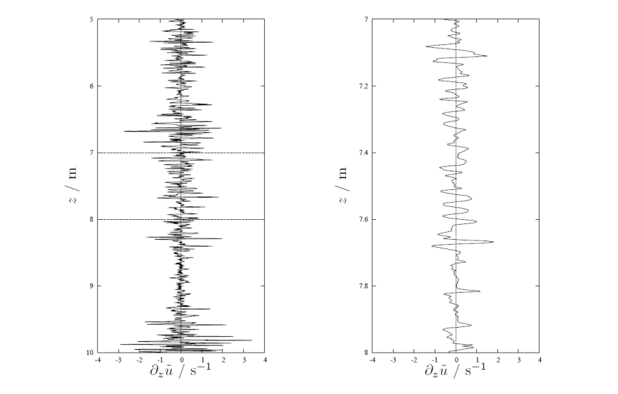
Fig. 9 Vertical shear of horizontal velocity measured by a freely falling shear microstructure profile in the mixed layer of the Northern Baltic Sea. Left panel: profile over a range of 5 m; right panel: enlarged vertgion of the same profile. Fig 1.7 from Umlauf and Burchard, 2020.#
Dissipation rate of TKE#
The dissipation rate of Turbulent Kinetic Energy (TKE) is derived from observations of shear gradients at the Kolmogorov microscale, \({(\frac{\nu^3}{\varepsilon})}^{{1/4}}\) through the following relation:
where \(\nu\) is molecular viscosity, a function of local temperature, \(\frac{\partial u'_i}{\partial x_j}\) is the turbulent shear along a component of \(i\) and \(j\) and the scale-factor \(\frac{15}{2}\) emerges from the assumption of isotropy given vertical turbulent fluctuations [Tay35](Taylor, 1935) (thus simplifying the 36 possible combinations of 9 terms taken 2 at a time).
An implicit assumption is Taylor’s “Frozen Turbulence Hypothesis”:
Dissipation is then statistically approximated by taking the integral of the shear spectrum between observed wavenumbers that are unaffected by instrument noise (typically between 1-100 cpm). Quality of the data is checked by fitting to an empirically derived Nasmyth spectra (1970) [Nas70], recently updated using a vastly larger dataset to the Lueck spectrum [Lue22].
At very strong dissipation rates, \(10^{-4}\) m\(^2\) s\(^{-3}\), the Kolmogorov microscale, \(L_k \propto \frac{1}{\varepsilon}\), becomes very small and shear microstructure probes may not capture the full shear spectrum. At very low dissipation rates, the signal to noise ratio may be too small to resolve reliable estimates of turbulence dissipation.
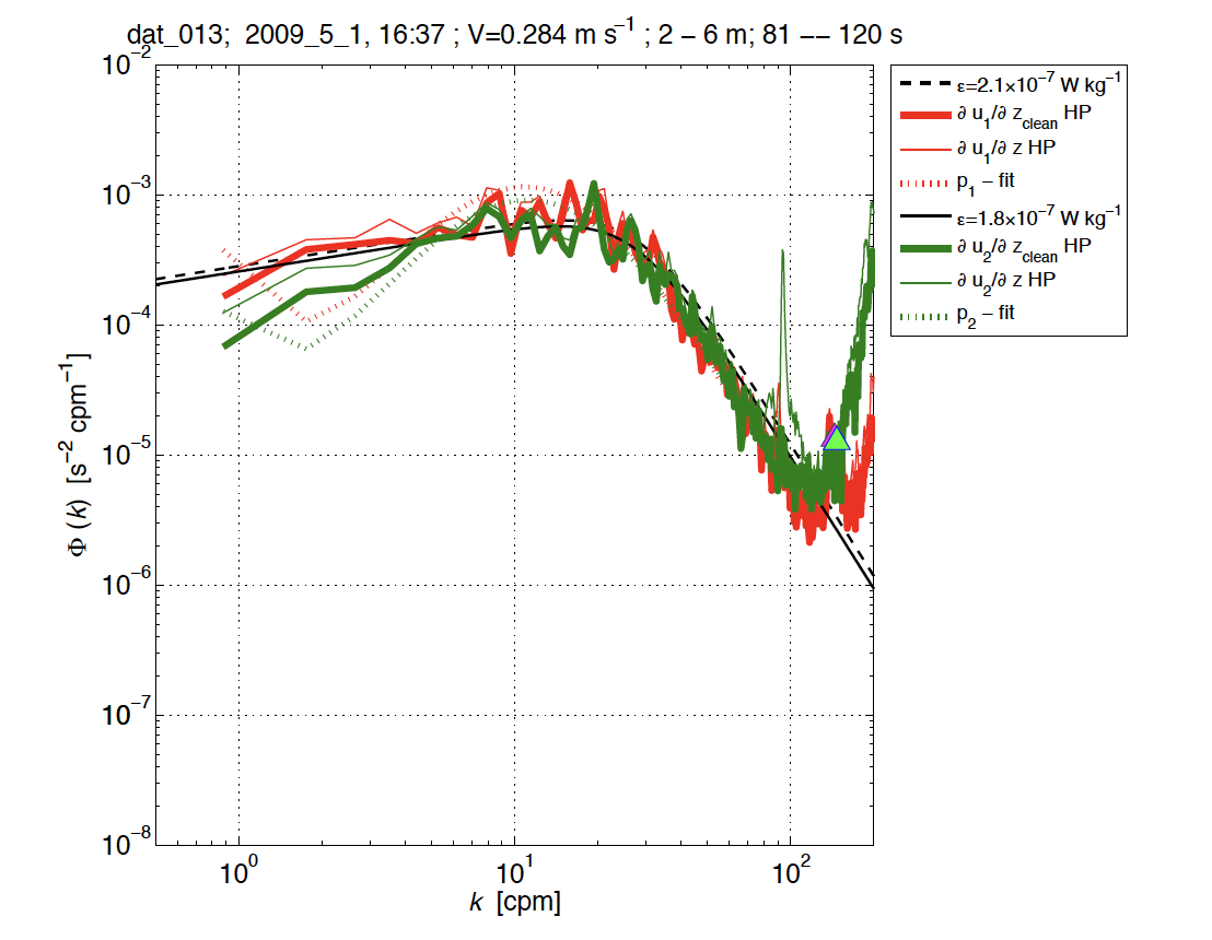
Fig. 10 The spectra of two components of along-path shear. Nasmyth spectra are overlain in black. Source: RSI Technical Note 028#
It is also possible to derive turbulence dissipation rates from temperature microstructure (following the Batchelor spectrum, [OC17], [BLI+17]) and conductivity microstructure.
Turbulent Fluxes#
Parcels of fluid with different properties are physically moved by turbulent eddies. The net flux is the result of averaging the transport by all of the eddies over a given area. The transfer of a property by turbulent eddies is usually represented through a paramterization that relates the turbulent eddies to the mean property gradient with an additional term referred to as eddy viscosity, K_m for momentum fluxes and eddy diffusivity, K_s for scalar fluxes. \(K_m\) is not nessecarily equivalent to \(K_s\). K_z is often used to denote vertical eddy diffusivity.
Heat Flux
where \(\rho_0\) is a reference density and \(C_p\) is the heat capacity of sea water, typically 4000 JK\(^{-1}\)kg \(^{-1}\).
Similarly,
Salt Flux
Buoyancy Flux
where \(b=-g\frac{\rho}{\rho_0}\).
Stress
Vertical Eddy Diffusivity#
\(K_z\) must be parameterized. One method in observational oceanography is the Osborn method (1980) [Osb80].
Recall the TKE budget equation assuming steady, homogeneous, 1D stratified shear flow, \(i=1,j=3\):
\(\varepsilon\) can be derived from measurements of microstructure shear using shear probes.
Buoyancy production/consumption is equivalently representative of the rate of change of Potential Energy.
Given the relation \(- K_z \frac{dB}{dz}\) where \(\frac{dB}{dz} = \frac{g}{\rho_p}\frac{d\rho}{dz}\), \(- K_z \frac{dB}{dz}\) = \(- K_z N^2\).
\(K_z\) can be derived as \(f({\varepsilon, Ri_f, N^2})\)
The flux richardson number represents the ratio of the rate of energy loss by work against stratification (rate of change of buoyancy with depth) to the rate of energy production by stress.
With some manipulation we get:
where \(\frac{\mathrm{Ri_f}}{1-\mathrm{Ri_f}} = \Gamma\), referred to as the efficiency factor, \(\Gamma\), is generally assumed to be 0.2, representing the conversion efficiency of TKE into PE of the system. Note, that while \(\Gamma\) is commonly assumed constant, it varies depending on the dynamics of the system. e.g. \(\Gamma\) < 0.2 (decrease in mixing efficiency) under intense mixing conditions due to weak gradients; \(\Gamma\) > 0.2 where double diffusive convection is possible because the source of turbulence production is dominated by a destabilizing buoyancy flux.
Thus:
which can be derived from observations.