What is turbulence

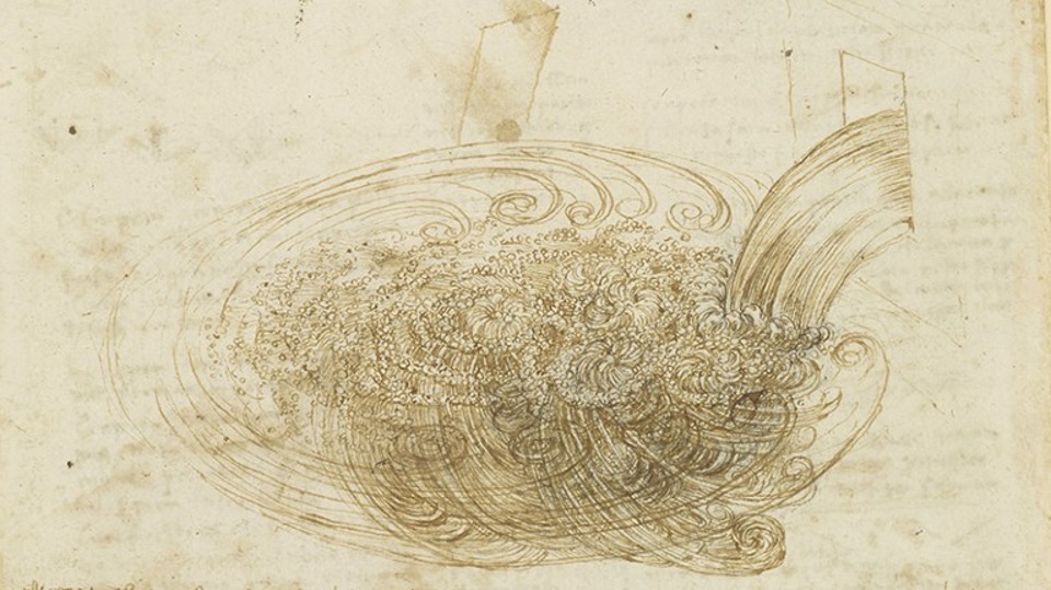
Fig. 1 Leonardo da Vinci’s “Studies of water” (c.1510-12). The term “turbulence” appears to have first been used in reference to fluid flows by da Vinci, who studied the phenomenon extensively

Turbulence in the ocean is responsible for the transport of fluid properties and the smoothing of gradients (dissipation of energy).

Turbulent mixing

Turbulence is a stochastic flow phenomenon that may occur in various fluids and gases. Due to its random character and complexity a generally valid theory for turbulence is lacking and turbulence remains one of the major unsovled problems of classic physics. Nevertheless, turbulent flows can be described. Here, we will look at the description of turbulence in oceanic flows.

Turbulence results from the nonlinear nature of advection, which enables interactions between motions on different spatial scales. Consequently, an initial disturbance with a given characteristic length scale tends to spread to progressively larger and smaller scales. This expansion is limited at large scales by boundaries and at small scales by viscosity.

By deforming a fluid, via stirring and strain, gradients are increased thus increasing the area available for molecular diffusion which occurs at small scales (the Kolmogorov length scale), effectively increasing the rate of mixing by several orders of magnitude (see Fig 2). In the case of a tracer, after mixing, variance is reduced.

The rate of molecular diffusion (kinematic viscosity, \(\nu\)) is \(\nu \approx 10^{-6} \text{ m}^2/\text{s}\).

The rate of eddy viscosity (turbulent diffusion, \(\nu_t\)) is \(\nu_t \approx 10^{-4} - 10^{-1} \text{ m}^2/\text{s}\).

Take note, kinematic viscosity if a property of the fluid, while eddy viscosity is a property of the flow.

A common analogy is that of mixing coffee and milk.

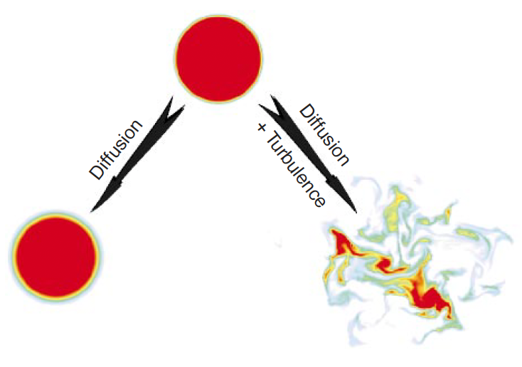
Fig. 2 A comparison of mixing enhanced by turbulence with mixing due to molecular processes alone, as revealed by a numerical solution of the equations of motion. The initial state includes a circular region of dyed fluid in a white background. Two possible evolutions are shown: one in which the fluid is motionless (save for random molecular motions), and one in which the fluid is in a state of fully developed, two-dimensional turbulence. The mixed region (yellow-blue) expands much more rapidly in the turbulent case. Smyth and Moum 2009 [SM09].

The energy cascade

Big whirls have little whirls that feed on their velocity,
And little whirls have lesser whirls and so on to viscosity - in the molecular sense.
- Richardson, 1922

Turbulence in the ocean is generated by large-scale forcing mechanisms, e.g. winds, tides, bottom friction, geothermal energy, Ocean generated, turbulence is transferred to smaller scales. At large scales, the flow is dominated by balanced forces (geostrophic balance), which tend to follow an inverse cascade. But, at fronts, instabilities can form, transferring energy to smaller scales via eddies. At the inertial subrange, energy transfer is governed by an approximate equilibrium, where large eddies break into smaller ones without loss of energy. Once turbulent eddies reach dissipative scales (the Kolmogorov Microscale, \({(\frac{\nu^3}{\varepsilon})}^{{1/4}}\)), molecular viscosity begins to play a dominant role and kinetic energy is converted into heat. This dissipation balances the energy input at large scales, maintaining a steady-state regime.

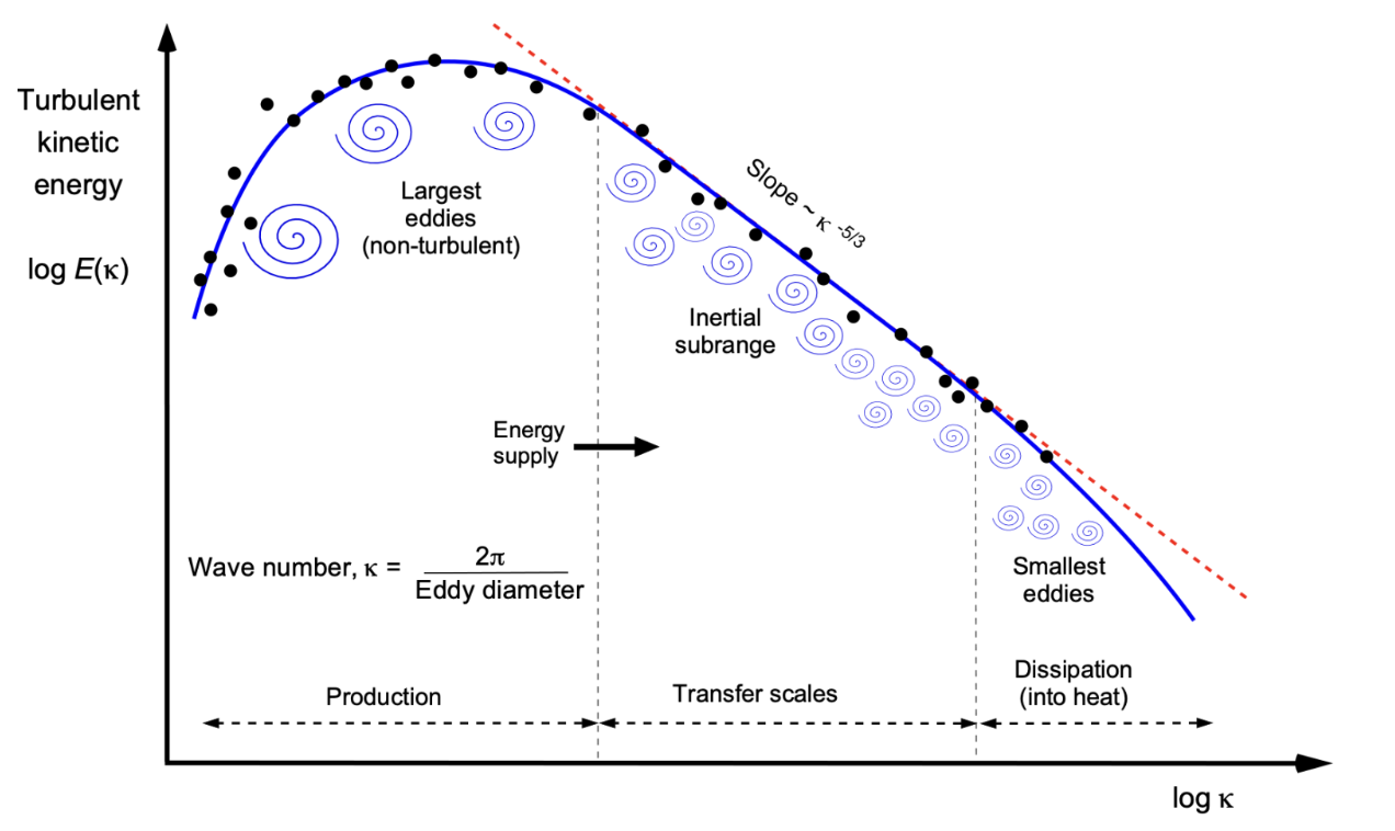
Fig. 3 The kinetic energy spectra of turbulence ranging from large scales to dissipative scales. \(E=q\varepsilon^{2/3}k^{-5/3}\), where \(k\) is an eddy wavenumber and \(q=0.5\), a universal constant. Source of schematic: Embry-Riddle Aeronautical University

Turbulent fluxes

Parcels of fluid with different properties are physically moved by turbulent eddies. Flux is defined as the total rate of flow of ‘stuff’ across or through a surface. The net flux is the result of averaging the transport by all of the eddies over a given area. Fluxes are often down-gradient (from high to low).

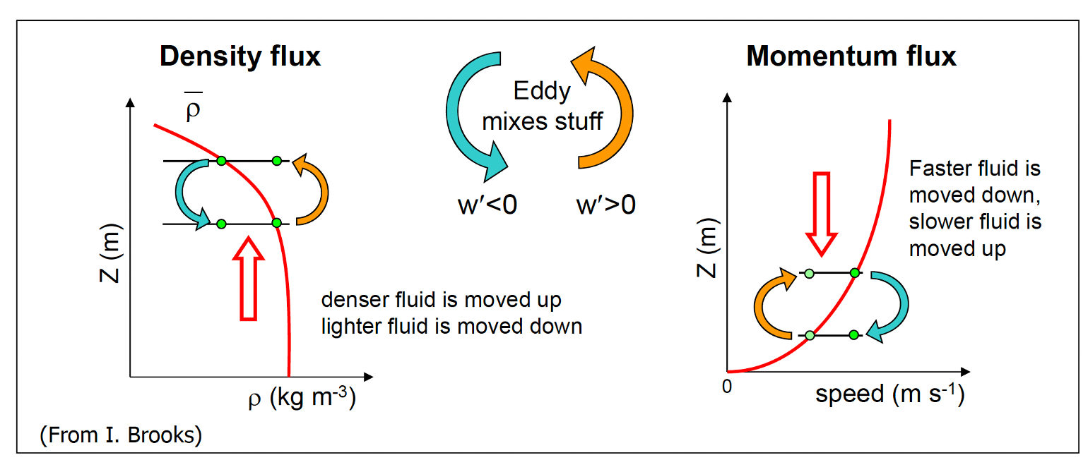
Fig. 4 The turbulent flux of momentum and scalars.

Definition of turbulence

It is difficult to provide a precise definition of turbulence. But it can be qualitatively described by properties that are common to all turbulent flows.

1. Randomness: Turbulent flows generate stochastic data sets both in time and in space. Small uncertainties in the initial and boundary conditions quickly amplify, rendering a deterministic description of individual turbulent fluctuations impossible. Turbulence can be described statistically (statistical moments, correlations, probability distributions).

2. Increased Transport and Mixing: Turbulent flows generally show strongly increased mixing and transport rates of matter, heat, and momentum because of the generation of sharp gradients and increased contact surfaces due to the complex strain field associated with the turbulent motions.

3. Vorticity: Turbulent flows are characterized by vorticity, manifested in the omnipresence of eddying motions. These vortices (“eddies”) involve a wide range of spatial wavelengths, ranging from the largest scales imposed by the bounding geometry down to the smallest scales, where eddies are dissipated due to molecular (viscous) smoothing. 3D.

4. Dissipative: Turbulence is “dissipative,” meaning the kinetic energy is dissipated into heat due to viscous friction at the smallest scales. Similarly, scalar fluctuations are smoothed by molecular diffusion, implying that the overall scalar variance is reduced. Thus, a mechanism must exist to transport energy and scalar variance from the largest scales, where they are introduced to the system, towards the smallest scales, where they are dissipated (broad energy spectrum).