Assignment: The observation and interpretation of turbulence dissipation#
The goal of the accompanying assignment is to become familiar with working with and interpreting observations of the rate of dissipation of turbulence.
The assignment is presented in Python, and while any coding language of preference can be used, the easiest would be to ensure that you have an updated version of python working on your local machine with the following dependencies: numpy, scipy, matplotlib, pandas, xarray (including h5netcdf) and gsw.
An environment.yml file is provided in the folder assignments which will install all nessecary dependencies provided you have the Anaconda distribution installed.
From your terminal, run conda env create -f environment.yml, then conda activate turbulence
Check that the python packages required are installed and adjust paths to your local machine if needed.
Completion and submission of the assignment is nessecary for completing the course.
Turbulent flow is ubiquitous, but not homogeneously distributed.
One method for observing turbulence is the observation of microstructure shear, from which the rate of turbulence dissipation can be directly computed. Such observations are crucial for understanding the contributions of various sources of turbulence production in the ocean, the turbulence flux of properties and the processes by which TKE is dissipated.
In this assignment, you will become familiar with the analysis of profiles of the dissipation rate of TKE under a range of forcing conditions.
Best practices for the processing of microstructure shear data are described in [LFB+24] with benchmark datasets described by [FDLBL24].
import numpy as np
import matplotlib.pyplot as plt
import xarray as xr
import pandas as pd
import gsw
# A function we will use later

def Nasfunc(x,eps,vis=1.6e-6):
    """ out=Nasfunc(x,eps,vis)
     x is the wavenumber, eps is the dissipation
     returns the Nasmyth's dissipation spectrum.
     The function form is given in Lueck et
     J. Oceanogr. 2002.
     default vis=1.6e-6 #m2/s kinematic viscocity
     See also Nasfunc_log"""

    ks = (eps*(vis**-3))**(1/4)
    x1= x/ks

    #fit provided by Fabian Wolk -see Lueck et al paper in J. Oceanogr. 2002
    G=(8.05*(x1**(1/3))) / (1+ ((20*x1)**3.7))
    return ((ks**2)*((eps*(vis**5))**(1/4)))*G   #in s-2/cpm
Part I#
Become familiar with the observation of microstructure shear
Baltic Sea - A quiescent region#
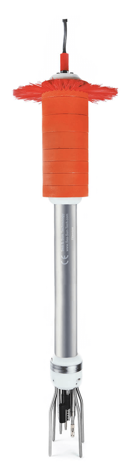
Fig. 23 A Sea and Sun Technology Microstructure Probe.#
This dataset can be downloaded here:
Holtermann, P. ATOMIX shear probes benchmark data: Example microstructure data from a Sea & Sun Technology MSS microstructure profiler, Bornholm Basin, Baltic Sea. NERC EDS British Oceanographic Data Centre NOC., https://doi.org/10.5285/0e35f96f-57e3-540b-e063-6c86abc06660 (2024).
The Baltic Sea profile was taken in September 2008 in the Bornholm Basin from the Research Vessel Poseidon. The oceanographic context and a detailed analysis of the data collected during this cruise are given in van der Lee and Umlauf (2011). The total depth was about 85 m. The instrument used was a MSS-Microstructure profiler with the serial number 38, produced by Sea & Sun Technology, Germany. It was equipped with two randomly oriented shear probes, one FP07 thermistor, and one PT100 temperature sensor and a conductivity cell for precision temperature and salinity measurements. The probe was also fitted with a vibration sensor, which is similar in design to a shear probe sensor, except that the airfoil is replaced by a small mass and is mounted inside the probe. The probe was connected with a cable to a ship-board data acquisition system and was operated with an electrical winch from the stern of the ship. During the profiling, the ship slowly moved along a transect with a speed of approximately 0.5 m s−1. The transect was oriented such that wind and surface currents came from the bow, such that the loosely tethered cable was always at a safe distance to the ship’s propeller. Using a sensor protection cage, it was possible to obtain nearly full-depth vertical profiles to within 0.1 m above the seafloor, with a descent speed of approximately 0.5 m s−1 .
First we will take a look at a few metrics to get familiar with dissipation data
# The data is stored as a grouped NetCDF file.
# First look at the global attributes.
dat_b=xr.open_dataset('assignment/baltic/MSS_Baltic.nc', engine="h5netcdf",group="")
dat_b.attrs
{'title': 'Example microstructure data from a Sea & Sun Technology MSS microstructure profiler',
 'summary': 'Vertical microstructure profile',
 'comment': 'The profile was collected on 20-Sep-2008 during the cruise POS373 onboard R.V. Poseidon, using the tethered free-fall MSS90-L profiler (Sea & Sun Technology, Germany, SN038). The dissipation rate was measured using two airfoil shear probes. In addition a fast-response FP07 thermistor, pressure, temperature, conductivity, vibration and oxygen sensors were mounted. All sensor were sampled with 1024 Hz. The processing of the data and the format of this data set follows the recommendations and guidelines of the SCOR Working Group #160, ATOMIX (https://wiki.uib.no/atomix). The netCDF file includes four hierarchical groups, corresponding to the four levels of microstructure data in the ATOMIX format. L1_converted : time series from all sensors converted into physical units L2_cleaned : selected signals that are filtered and/or despiked before spectral analysis. Time stamp and length of the signals are the same as in L1. L3_spectra : wavenumber spectra from shear probes and vibration sensors L4_dissipation: dissipation estimates together with quality control parameters L2_cleaned time series used for spectral analysis are marked with section numbers.',
 'platform_type': 'research vessel',
 'creation_time': '2024-01-17T15:18:42Z',
 'date_update': '2024-01-17T15:18:42Z',
 'date_created': '2024-01-17',
 'time_reference_year': np.float64(2008.0),
 'fs_fast': np.float64(1024.0),
 'fs_ctd': np.float64(1024.0),
 'profiling_direction': 'vertical',
 'HP_cut': np.float64(0.15),
 'despike_shear_fraction_limit': np.float64(0.05),
 'FOM_limit': np.float64(1.15),
 'despike_iterations_limit': np.float64(8.0),
 'diss_ratio_limit': np.float64(2.77),
 'variance_resolved_limit': np.float64(0.5),
 'fft_length': np.float64(2048.0),
 'diss_length': np.float64(5120.0),
 'overlap': np.float64(2560.0),
 'goodman': np.float64(1.0),
 'geospatial_lat_min': np.float64(55.235416666666666),
 'geospatial_lat_max': np.float64(55.235416666666666),
 'geospatial_lon_min': np.float64(15.978098333333334),
 'geospatial_lon_max': np.float64(15.978098333333334),
 'geospatial_vertical_min': np.float64(0.0),
 'geospatial_vertical_max': np.float64(88.0),
 'geospatial_vertical_positive': 'down',
 'time_coverage_start': '2008-09-20T10:50:04Z',
 'time_coverage_end': '2008-09-20T10:52:49Z',
 'conventions': 'CF-1.6, ACDD-1.3, ATOMIX',
 'history': 'v2.2',
 'data_mode': 'D',
 'area': 'western Baltic Sea',
 'principal_investigator': 'Lars Umlauf',
 'institution': 'Leibniz Institute for Baltic Sea Research, Warnemuende',
 'references': 'E. M. van der Lee and L. Umlauf, Internal wave mixing in the Baltic Sea: Near-inertial waves in the absence of tides, Journal of Geophysical Research: Oceans, vol. 116, no. C10, Oct. 2011, doi: 10.1029/2011JC007072.',
 'authors': 'E. M. van der Lee and L. Umlauf',
 'contact': 'lars.umlauf@io-warnemuende.de',
 'project_name': 'SHIC',
 'cruise': 'POS373',
 'vessel': 'RV Poseidon',
 'creator_name': 'Peter Holtermann',
 'creator_email': 'peter.holtermann@io-warnemuende.de',
 'license': 'http://creativecommons.org/licenses/by/4.0/',
 'citation': 'Holtermann, Peter (2024). ATOMIX shear probes benchmark data: Example microstructure data from a Sea & Sun Technology MSS microstructure profiler, Bornholm Basin, Baltic Sea. British Oceanographic Data Centre. DOI: 10.5285/0e35f96f-57e3-540b-e063-6c86abc06660',
 'DOI': '10.5285/0e35f96f-57e3-540b-e063-6c86abc06660'}
# open each group separately

dat_bL1=xr.open_dataset('assignment/baltic/MSS_Baltic.nc', engine="h5netcdf",group="L1_converted")
dat_bL2=xr.open_dataset('assignment/baltic/MSS_Baltic.nc', engine="h5netcdf",group="L2_cleaned")
dat_bL3=xr.open_dataset('assignment/baltic/MSS_Baltic.nc', engine="h5netcdf",group="L3_spectra")
dat_bL4=xr.open_dataset('assignment/baltic/MSS_Baltic.nc', engine="h5netcdf",group="L4_dissipation")
dat_bL4
<xarray.Dataset> Size: 13kB
Dimensions:         (TIME_SPECTRA: 61, N_SHEAR_SENSORS: 2)
Dimensions without coordinates: TIME_SPECTRA, N_SHEAR_SENSORS
Data variables: (12/16)
    TIME            (TIME_SPECTRA) datetime64[ns] 488B ...
    EPSI            (N_SHEAR_SENSORS, TIME_SPECTRA) float64 976B ...
    EPSI_FINAL      (TIME_SPECTRA) float64 488B ...
    SECTION_NUMBER  (TIME_SPECTRA) float64 488B ...
    PSPD_REL        (TIME_SPECTRA) float64 488B ...
    PRES            (TIME_SPECTRA) float64 488B ...
    ...              ...
    EPSI_STD        (N_SHEAR_SENSORS, TIME_SPECTRA) float64 976B ...
    N_S             (N_SHEAR_SENSORS, TIME_SPECTRA) float64 976B ...
    KMAX            (N_SHEAR_SENSORS, TIME_SPECTRA) float64 976B ...
    KMIN            (N_SHEAR_SENSORS, TIME_SPECTRA) float64 976B ...
    EPSI_FLAGS      (N_SHEAR_SENSORS, TIME_SPECTRA) float64 976B ...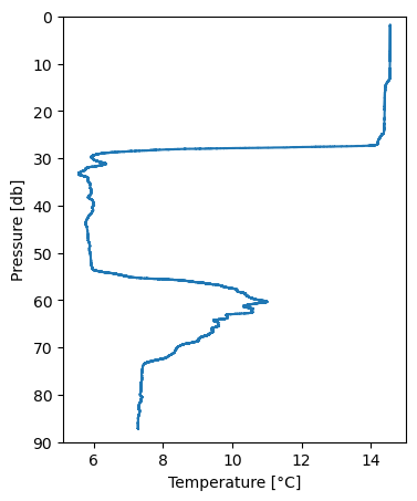
METHOD (N_SHEAR_SENSORS, TIME_SPECTRA) float64 976B ...Plot vertical profile of temperature#
1.1 Describe what you can about the hydrographic structure from this plot. Can refer to [VdLU11] for context.
plt.figure(figsize=(4,5))
plt.plot(dat_bL1.TEMP_CTD,dat_bL1.PRES)
plt.ylim(90,0)
plt.ylabel('Pressure [db]')
plt.xlabel('Temperature [°C]')
Text(0.5, 0, 'Temperature [°C]')
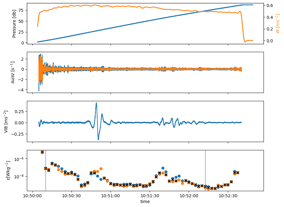
Plot time series#
Below are time series of a) Pressure and Velocity through water, b) vertical shear, c) platform vibrations and d) turbulence dissipation rate.
1.2) Interpret what might be causing enhanced vibrations in c.
1.3a) Describe the vertical profile of the dissipation rate of turbulence (where dissipation rate is high, where it is low) with reference to the distance from the surface and the temperature profile.
1.3b) Select two points, one with high dissipation rate and one with low dissipation rate and overlay vertical lines at these chosen points in subpanels d).
fig,ax=plt.subplots(4,1,figsize=(10,8),sharex=True)

ax[0].plot(dat_bL1.TIME,dat_bL1.PRES,lw=2)
ax[0].set_ylabel('Pressure [db]')

axa=ax[0].twinx()
axa.plot(dat_bL1.TIME,dat_bL1.PSPD_REL,c='tab:orange',lw=2)
axa.set_ylabel('W [ms$^{-1}$]',c='tab:orange')


ax[1].plot(dat_bL2.TIME,dat_bL2.SHEAR[0,:])
ax[1].plot(dat_bL2.TIME,dat_bL2.SHEAR[1,:])

ax[1].set_ylabel(r'$\partial u / \partial z$ [s$^{-1}$]')

ax[2].plot(dat_bL2.TIME,dat_bL2.VIB[0,:])
ax[2].set_ylabel(r'VIB [ms$^{-2}$]')


ax[3].scatter(dat_bL4.TIME,dat_bL4.EPSI[0,:],label=r'$\epsilon_1$')
ax[3].scatter(dat_bL4.TIME,dat_bL4.EPSI[1,:],label=r'$\epsilon_2$')
ax[3].scatter(dat_bL4.TIME,dat_bL4.EPSI_FINAL,c='k',marker='x',label=r'$\epsilon$')


### EDIT HERE, only dummies used
# 1.3b: identify two regions of dissipation (strong versus quiescent)
i= 1   # strong dissipation
j= 50   # weak dissipation

ax[3].axvline(pd.to_datetime(dat_bL4.TIME[i].values),c='grey',lw=1)
ax[3].axvline(pd.to_datetime(dat_bL4.TIME[j].values),c='grey',lw=1)

ax[3].set_yscale('log')
ax[3].set_ylabel(r'$\epsilon \mathrm{[W kg^{-1}]}$')
ax[3].set_xlabel('time')
Text(0.5, 0, 'time')
Create model Nasmyth Spectra for chosen dissipation rates in the data#
1.4) Using the Nasmyth model, create spectra for your selected dissipation rates.
# print dissipation values for chosen spectra and create model nasmyth shear spectra

knas_strong = np.linspace(0,100,len(dat_bL3.KCYC[:,i]))
print(dat_bL4.EPSI_FINAL[i])
nasmyth_strong = Nasfunc(knas_strong,dat_bL4.EPSI_FINAL[i].values)

print(dat_bL4.EPSI_FINAL[j])
knas_weak = np.linspace(0,100,len(dat_bL3.KCYC[:,j]))
nasmyth_weak = Nasfunc(knas_weak,dat_bL4.EPSI_FINAL[j].values)
<xarray.DataArray 'EPSI_FINAL' ()> Size: 8B
array(7.880893e-08)
Attributes:
    standard_name:  specific_turbulent_kinetic_energy_dissipation_in_sea_water
    units:          W kg-1
    long_name:      dissipation rate of turbulent kinetic energy per unit mas...
<xarray.DataArray 'EPSI_FINAL' ()> Size: 8B
array(6.033673e-10)
Attributes:
    standard_name:  specific_turbulent_kinetic_energy_dissipation_in_sea_water
    units:          W kg-1
    long_name:      dissipation rate of turbulent kinetic energy per unit mas...
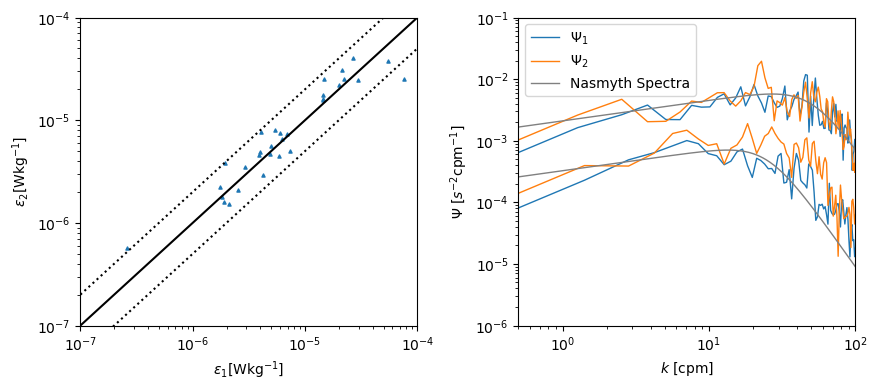
Dissipation estimates from shear spectra#
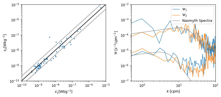
Look at the agreement between dissipation estimates from the two spectra. Generally, turbulence can be observed to within a factor of two [MGLC95].
1.5) Plot shear spectra at the two dissipation rates that you chose earlier. How does shear spectra relate to dissipation rates?
fig,ax=plt.subplots(1,2,figsize=(10,4))
fig.subplots_adjust(wspace=0.3)

## Dissipation plot

ax[0].scatter(dat_bL4.EPSI[0,:],dat_bL4.EPSI[1,:],marker='^',s=5)

ax[0].set_yscale('log')
ax[0].set_xscale('log')

# Define the range for the 1-to-1 and confidence interval lines
x_vals = np.logspace(-10,
                     -5, 100)

# Plot 1:1 line
ax[0].plot(x_vals, x_vals, 'k')

# Plot factor of 2 confidence intervals
ax[0].plot(x_vals, 2 * x_vals, 'k:')
ax[0].plot(x_vals, 0.5* x_vals, 'k:')

ax[0].set_ylim(1e-10,1e-5)
ax[0].set_xlim(1e-10,1e-5)

ax[0].set_xlabel(r'$\epsilon_1 \mathrm{[W kg^{-1}]}$')
ax[0].set_ylabel(r'$\epsilon_2 \mathrm{[W kg^{-1}]}$')


## Spectra

ax[1].plot(dat_bL3.KCYC[:,i],dat_bL3.SH_SPEC_CLEAN[0,:,i],c='tab:blue',lw=1,label=r'$\Psi_{1}$')
ax[1].plot(dat_bL3.KCYC[:,i],dat_bL3.SH_SPEC_CLEAN[1,:,i],c='tab:orange',lw=1,label=r'$\Psi_{2}$')
ax[1].plot(knas_strong,nasmyth_strong,c='grey',lw=1,label='Nasmyth Spectra')

ax[1].plot(dat_bL3.KCYC[:,j],dat_bL3.SH_SPEC_CLEAN[0,:,j],c='tab:blue',lw=1)
ax[1].plot(dat_bL3.KCYC[:,j],dat_bL3.SH_SPEC_CLEAN[1,:,j],c='tab:orange',lw=1)
ax[1].plot(knas_weak,nasmyth_weak,c='grey',lw=1)

ax[1].set_yscale('log')
ax[1].set_xscale('log')

ax[1].set_xlim(0.5,1e2)
ax[1].set_ylim(1e-7,1e-2)

ax[1].legend()

ax[1].set_xlabel(r'$k$ [cpm]')
ax[1].set_ylabel(r'$\Psi$ $[s^{-2}\mathrm{cpm}^{-1}]$')
Text(0, 0.5, '$\\Psi$ $[s^{-2}\\mathrm{cpm}^{-1}]$')
Haro Straight - A tidal channel.#
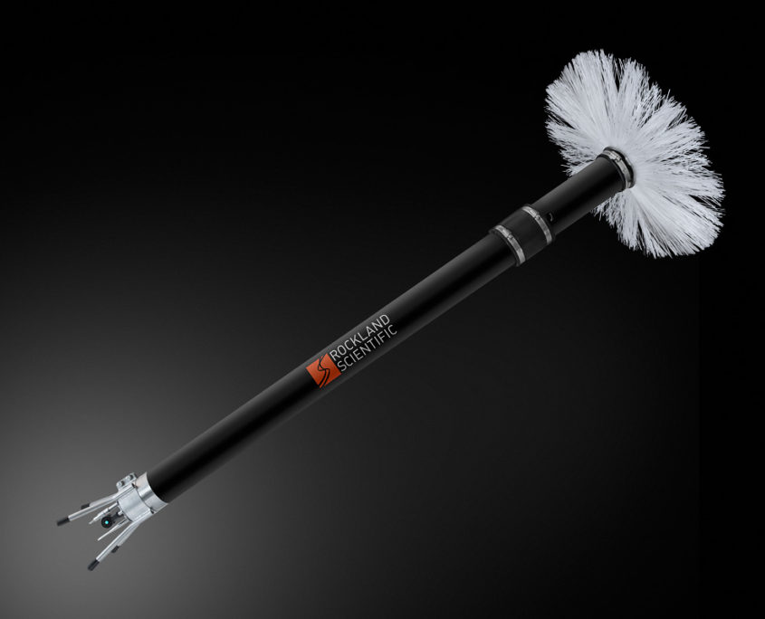
Fig. 24 A Rockland Scientific VMP250.#
This dataset can be downloaded here:
Lueck, R. ATOMIX shear probes benchmark data: a dissipation profile from Haro Strait, British Columbia, Canada obtained with a vertical microstructure profiler in October 2016. NERC EDS British Oceanographic Data Centre NOC., https://doi.org/10.5285/0ec16a65-abdf-2822-e063-6c86abc06533 (2024).
This turbulence profile was taken in a side channel adjacent to Haro Strait on the east coast of Vancouver Island, British Columbia, Canada, on 19 October 2016. The instrument was a VMP-250-IR (internally recording and serial number 215) vertical profiler from Rockland Scientific, Canada. It was configured to collect data while descending, with two shear probes oriented to measure two orthogonal components of the vertical shear of horizontal current, one FP07 thermistor, and two vibration sensors, all of which were anti-alias low-pass filtered at 98 Hz and sampled at a rate of 512 s−1.
# First look at the global attributes
dat_h=xr.open_dataset('assignment/haro_straight/VMP250_TidalChannel_024.nc', engine="h5netcdf",group="")
dat_h.attrs
{'authors': 'Rolf Lueck',
 'type': 'Time series from a VMP',
 'source': 'VMP-250',
 'platform_type': 'Research Vessel',
 'title': 'ATOMIX shear probes benchmark data: a dissipation profile from Haro Strait, British Columbia, Canada obtained with a vertical microstructure profiler in October 2016',
 'summary': 'This file was processed using a speed equal to the rate-of-change of pressure. The profile was collected using a tethered free-fall vertical microstructure profiler (VMP-250IR, Rockland Scientific, Canada), prepared as a benchmark shear-probe data example for the Scientific Committee on Oceanographic Research (SCOR) Working Group #160, "Analyzing ocean turbulence observations to quantify mixing" (ATOMIX, https://wiki.uib.no/atomix). The profile was collected on 2016-10-19 17:49:11 from R.V. Strickland in Haro Strait for a demonstration class. The bottom depth at this location is approximately 80 meters. The dissipation rate was measured using two airfoil shear probes. The dataset has been processed and formatted in accordance with ATOMIX guidelines and recommendations. The provided file is organized in four hierarchical groups including continuous time series of data converted into physical units, cleaned time series used for spectral analysis, wavenumber spectra, and dissipation rate estimates. For more detailed information, please refer to the comments within the data file.',
 'comment': 'The profile was collected on 2016-10-19 17:49:11 in Haro Strait to demonstrate to a class of student how one uses a vertical downward-profiling microstructure instrument. Additional sensors include one fast-response FP07 thermistor and a SBE micro-conductivity sensor, a 2-axis vibration sensor, a pressure transducer, a 2-axis inclinometer, and a high-accuracy JAC temperature and conductivity. The turbulence and acceleration channels were sampled at a rate of 512 Hz, while the other channels were sampled at 64 Hz.\n\tThe processing of the data and the format of this data set follows the recommendations and guidelines of the SCOR Working Group #160, ATOMIX (https://wiki.uib.no/atomix). The processing was based on the standard Matlab routines provided by Rockland Scientific, which were adjusted for the ATOMIX recommendations. The netCDF file includes four hierarchical groups, corresponding to the four levels of microstructure data in the ATOMIX format.\n\tL1_converted : time series from all sensors converted into physical units. \n\tL2_cleaned : selected signals that are filtered and/or de-spiked before spectral analysis. Time stamp and length of the signals are the same as in L1. \n\tL3_spectra : wavenumber spectra from shear probes and vibration sensors. \n\tL4_dissipation: dissipation estimates together with quality control parameters. \n\tL2_cleaned time series used for spectral analysis are marked with section numbers. A section (a more general term for a profile) is a continuous segment of the time series with dissipation estimates. There is only 1 section (profile) in this example data set. Spectra (L3) and dissipation rate (L4) estimates are given only for this one section. Choices of filter and de-spiking parameters and various thresholds for quality assurance are given in the global attributes. Spectral calculation and dissipation rate estimate details are given in the attributes and processing parameters. \n\tL3 includes the cyclic wavenumber spectra obtained using half-overlapping record lengths of 5 s and FFT lengths of 1 s that are cosine windowed and overlapped by 50%. Vibration-coherent noise is removed using the method of Goodman et al. (2006). Shear and vibration spectra, and the cleaned shear spectra using the Goodman method are provided. \n\tL4 includes estimates from both shear probes, using the cleaned spectra, as well as a final estimate (average over estimates that passed the quality checks), together with quality control parameters. The figure of merit (FOM) and mean absolute deviation (MAD) relative to the Lueck model spectrum are used. Data quality flags for dissipation estimates are summarized in the attributes of the variable EPSI_FLAGS in the L4 group. A final dissipation estimate, EPSI_FINAL, failing the data quality control is reported as NaN. However, the individual dissipation estimates from each probe are accessible in the EPSI parameter.',
 'acknowledgement': 'The support of the captain and crew of the RV Strickland is appreciated.',
 'citation': 'Lueck, Rolf, (2024). ATOMIX shear probes benchmark data: a dissipation profile from Haro Strait, British Columbia, Canada obtained with a vertical microstructure profiler in October 2016. NERC EDS British Oceanographic Data Centre NOC. doi:10.5285/0ec16a65-abdf-2822-e063-6c86abc06533',
 'references': 'Goodman, L., Levine, E. R., and Lueck, R. G. (2006). On Measuring the Terms of the Turbulent Kinetic Energy Budget from an AUV, Journal of Atmospheric and Oceanic Technology, 23, 977\udce2\udc80\udc93990, https://doi.org/10.1175/JTECH1889.1, 2006. Lueck, R. G. (2022a). The statistics of oceanic turbulence measurements. Part 1: Shear variance and dissipation rates. Journal of Atmospheric and Oceanic Technology 39, 1259\udce2\udc80\udc931271. doi:10.1175/JTECH-D-21-0051.1 Lueck, R. (2022b). The statistics of oceanic turbulence measurements. Part 2: Shear spectra and a new spectral model. Journal of Atmospheric and Oceanic Technology 39, 1273\udce2\udc80\udc931282. doi:10.1175/JTECH-D-21-0050.1.',
 'institution': 'Rockland Scientific International, Inc.',
 'area': 'Haro Strait',
 'PI': 'Rolf Lueck',
 'contact': 'Rolf Lueck',
 'project_name': '',
 'cruise': '',
 'vessel': 'RV Strickland',
 'creation_time': '2024-01-19 13:55:54',
 'date_updated': '',
 'time_reference_year': np.float64(2016.0),
 'creator_name': 'Rolf Lueck',
 'creator_initials': 'RGL',
 'creator_email': 'rolf@rocklandscientific.com',
 'creator_url': '',
 'conventions': 'CF-1.6, ACDD-1.3, ATOMIX',
 'history': 'Version 1',
 'data_mode': 'D #(D)elayed',
 'geospatial_lat_min': np.float64(48.673),
 'geospatial_lat_max': np.float64(48.673),
 'geospatial_lon_min': np.float64(-123.368),
 'geospatial_lon_max': np.float64(-123.368),
 'keywords': 'turbulence, mixing, dissipation rate, shear probes',
 'license': 'http://creativecommons.org/licenses/by/4.0/',
 'instrument': 'VMP-250',
 'profiling_direction': 'down',
 'instrument_sampling_rate': np.float64(512.0),
 'instrument_serial_number': array([], dtype=float64),
 'despike_shear_fraction_limit': np.float64(0.05),
 'despike_shear_iterations_limit': np.float64(8.0),
 'diss_ratio_limit': np.float64(2.7718585822512662),
 'variance_resolved_limit': np.float64(0.6),
 'max_depth': np.float64(68.14594054397587),
 'fs_fast': np.float64(512.0327777777778),
 'fs_slow': np.float64(64.00409722222223),
 'date_created': '2024-01-19 13:55:54',
 'profile_dir': 'down',
 'time_coverage_start': '2016-10-19 17:50:44',
 'time_coverage_end': '2016-10-19 17:52:02',
 'FOM_limit': np.float64(1.15),
 'HP_cut': np.float64(0.4),
 'LP_cut': np.float64(30.0),
 'P_end': array([], dtype=float64),
 'P_start': array([], dtype=float64),
 'YD_0': np.float64(0.0),
 'despike_A': array([ inf, 0.5 , 0.04]),
 'despike_C': array([10.  ,  1.  ,  0.04]),
 'despike_sh': array([8.  , 0.5 , 0.04]),
 'despike_shear_limit': np.float64(0.05),
 'despike_shear_pass_limit': np.float64(8.0),
 'diss_length': np.float64(2560.0),
 'f_AA': np.float64(98.0),
 'f_limit': np.float64(inf),
 'fft_length': np.float64(512.0),
 'fit_2_isr': np.float64(1.5e-05),
 'fit_order': np.float64(3.0),
 'fname': 'VMP250_TidalChannel_024',
 'goodman': np.float64(1.0),
 'goodman_depth_range': array([  10., 1000.]),
 'goodman_fft_length': np.float64(2.0),
 'make_figures': np.float64(0.0),
 'op_area': 'open_ocean',
 'overlap': np.float64(1280.0),
 'plot_battery': np.float64(0.0),
 'plot_dissipation': np.float64(0.0),
 'plot_kinematics': np.float64(0.0),
 'plot_rawaccel': np.float64(0.0),
 'plot_sensors': np.float64(0.0),
 'plot_spectra': np.float64(0.0),
 'plot_spectrograms': np.float64(0.0),
 'profile_min_P': np.float64(3.0),
 'profile_min_W': np.float64(0.5),
 'profile_min_duration': np.float64(20.0),
 'profile_num': np.float64(1.0),
 'MF_extra_points': np.float64(0.0),
 'MF_k': np.float64(4.0),
 'MF_k_mag': np.float64(1.7),
 'MF_len': np.float64(256.0),
 'MF_st_dev': 'st_dev',
 'MF_threshold': array([], dtype=float64),
 'aoa': np.float64(0.0),
 'constant_speed': array([], dtype=float64),
 'constant_temp': array([], dtype=float64),
 'gradC_method': 'high_pass',
 'gradT_method': 'high_pass',
 'hotel_file': array([], dtype=float64),
 'speed_cutout': np.float64(0.05),
 'speed_tau': np.float64(1.5),
 'time_offset': np.float64(0.0),
 'vehicle': 'vmp',
 'dof_spec': np.float64(17.099999999999998),
 'num_fft_segments': np.float64(9.0),
 'fft_length_sec': np.float64(1.0),
 'diss_length_sec': np.float64(5.0),
 'overlap_sec': np.float64(2.5),
 'temperature_source': 'T1_fast',
 'speed_source': 'Rate of change of pressure',
 'ssetupfilestr': '; 2017-10-31 12:03:54 patched configuration string\n; Standard configuration setup.cfg file for a downward profiling VMP.\n; Change the vehicle type in the [instrument_info] section to rvmp for an\n;  uprising profiler.\n; Created by RSI, 2015-12-17\n; Modified by Andrew Bourget, 2016-09-19 with coefficients\n; Edited pressure coefficient to zero by subtracting 0.85 from coeff 0  2016-09-19 \n; Made for Victor\n; Changed Sh1 probe to M1111 2017_10_31\n;\n; Any line that starts with a semicolon, ";", is a comment and is ignored by \n;  software. Likewise, everything to the right of a semicolon is ignored.\n;  Use this feature to leave notes and to indicate that you have made changes \n;  to this file. Indicate the date (YYYY-MM-DD), your name and a brief \n;  description of your changes.\n\n; The first section is the [root] section. It determines the data \n;  acquisition parameters. It does not need to be declared explicitly.\n\nrate        = 512    ; the sampling rate of "fast" channels\nprefix      = VMP_   ; the base name of your data files. A 3-digit file number is \n\t\t\t\t\t ; appended to this base name. The limit is 8 characters\n                     ; total for internally recording instruments.\ndisk        = /data  ; the directory for the data files. It must exist. The directory \n\t\t\t\t\t ; should be /data for internally recording instruments. For \n\t\t\t\t\t ; real-time instruments it is best to leave this blank, so \n\t\t\t\t\t ; that it defaults to the local directory.\nrecsize     = 1      ; the size of a record in seconds\nman_com_rate= 3      ; the communication rate for real-time VMPs. This value must\n                     ; match the jumper settings of the RSTRANS in your VMP. \n                     ; It is not needed for internally recording instruments.\nno-fast     = 7      ; number of fast "columns" in the address matrix (see below).\nno-slow     = 2      ; number of slow "columns" in the address matrix.\n\n; -----------------\n;This section presents the address [matrix] of your instrument and \n;  automatically ends the [root] section above. The first columns are "slow"\n;  channels as defined by the "no-slow" parameter in the [root] section.\n;  The remainder are "fast" columns ("no-fast").\n[matrix]\nnum_rows=8\nrow01   =\t255\t0\t1\t2\t5\t8\t9\t64\t65\t\nrow02   =\t32\t40\t1\t2\t5\t8\t9\t64\t65\t\nrow03   =\t41\t42\t1\t2\t5\t8\t9\t64\t65\t\nrow04   =\t4\t0\t1\t2\t5\t8\t9\t64\t65\t\nrow05   =\t10\t11\t1\t2\t5\t8\t9\t64\t65\t\nrow06   =\t12\t48\t1\t2\t5\t8\t9\t64\t65\t\nrow07   =\t0\t49\t1\t2\t5\t8\t9\t64\t65\t\nrow08   =\t0\t50\t1\t2\t5\t8\t9\t64\t65\t\n\n; --------------------\n;This section identifies your instrument. Only the vehicle is important.\n[instrument_info]\nvehicle = vmp      ; downward profiling. Use either vmp or rvmp but not both.\n;vehicle= rvmp     ; upward profiling\nmodel   = vmp-250IR  ; The actual model. Used for trouble shooting.\nsn      = 215      ; The serial numnber of the instrument. For trouble shooting\n\n; --------------------\n; The next section is optional and can be expanded. Do not use the parameter "id = ".\n[cruise_info]\noperator    = \nproject     = 2017 Ocean Turbulence Workshop\nship        =\nleg         =\n\n; --------------------\n; Next come the [channel] sections. These are used to convert your data \n;  into physical units, and to save them into a mat-file. \n;  They also determine the name given to various signals \n;  in your data file. Please, stick to the convention of \n;  RSI because data visualization using the RSI Matlab Library of functions\n;  assumes particular names. However, data will be converted into physical\n;  units regardless of the name of the channels. If you change the names,\n;  then data visualization and further processing is your responsibility.\n;  A list of typical channel addresses (id) and their names and functions\n;  is at the end of this file.\n\n; Each channel section consists of a part that is unique to your instrument.\n;  It does not need to be changed. The second part is dependent on your \n;  sensors (shear probes, FP07 thermistors, etc.) and must be updated \n;  whenever you change a probe.\n;\n; The record average value is display for some channels with a real-time\n;  instrument. Display can be forced or suppressed using \n;  display = true, or display = false. Internally recording instruments\n;  have no display. The units used for display can be specified with\n;  units = [unit_symbols]. Keep it short for best display. \n\n; The ground reference channel.\n[channel]\n; instrument dependent parameters\nid      = 0   ; the channel address, 0 to 254.  Listed in the [matrix] section.\nname    = Gnd ; the name it will have in the mat-file.\ntype    = gnd ; the algorithm used to convert raw data into physical units.\n;coef0   = 0   ; the coefficients required for conversion. None in this case.\n\n; --------------\n; The piezo-vibration sensors\n[channel]\n; instrument dependent parameters\nid      = 1\nname    = Ax\ntype    = piezo\n\n[channel]\n; instrument dependent parameters\nid      = 2\nname    = Ay\ntype    = piezo\n\n; -----------------\n; The thermistor channels\n; without pre-emphasis\n[channel]\n; instrument dependent parameters\nid          = 4\nname        = T1\ntype        = therm\nadc_fs      = 4.096\nadc_bits    = 16\na           = -9.4\nb           = 0.9991\nG           = 6\nE_B         = 0.68222\n; sensor dependent parameters\nSN          = T1000\nbeta_1      = 2.6297e3\nbeta_2      = 1.9189e3\nT_0         = 281.9394\ncal_date    = 2017-10-31\nunits       = [C]\n\n; with pre-emphasis\n[channel]\n; instrument dependent parameter\nid          = 5\nname        = T1_dT1\ntype        = therm\ndiff_gain   = 0.925\n\n; -----------------\n; The shear probe channels\n[channel]\n; instrument dependent parameters\nid          = 8 \nname        = sh1\ntype        = shear\nadc_fs      = 4.096\nadc_bits    = 16\ndiff_gain   = 0.933\n; sensor dependent parameters\nsens        = 0.0716\nSN          = M1000\ncal_date    = 2016-09-07\n\n[channel]\n; instrument dependent parameters\nid          = 9\nname        = sh2\ntype        = shear\nadc_fs      = 4.096\nadc_bits    = 16\ndiff_gain   = 0.944\n; sensor dependent parameters\nsens        = 0.0705\nSN          = M1111\ncal_date    = 2016-09-07\n\n; -----------------\n; The pressure transducder\n; without pre-emphasis\n[channel]\n; instrument dependent parameters\nid          = 10\nname        = P\ntype        = poly\n; sensor dependent parameters\ncoef0       = -1.83303\ncoef1       = 0.029257\ncoef2       = 0\ncal_date    = 2016-09-07\nunits       = [dBar]\n\n; with pre-emphasis\n[channel]\n; instrument dependent parameters\nid          = 11\nname        = P_dP\ntype        = poly\ndiff_gain   = 20.29\n\n; pressure transducer voltage\n[channel]\n; instrument dependent parameters\nid      = 12\nname    = PV\ntype    = poly\ncoef0   = 4.096\ncoef1   = 1.25e-4\nunits   = [V]\n\n; -----------------\n; Battery voltage or power supply voltage\n[channel]\n; instrument dependent parameters\nid          = 32\nname        = V_Bat\ntype        = voltage\nG           = 0.1\nadc_fs      = 4.096\nadc_bits    = 16\nunits       = [V]\n\n; -----------------\n; The ADIS precision inclinometer with built in thermometer\n[channel]\n; instrument dependent parameters\nid      = 40\nname    = Incl_Y\ntype    = inclxy\n; sensor dependent parameters\ncoef0   = 0\ncoef1   = 0.025\nunits   = [deg]\n\n[channel]\n; instrument dependent parameters\nid      = 41\nname    = Incl_X\ntype    = inclxy\n; sensor dependent parameters\ncoef0   = 0\ncoef1   = 0.025\nunits   = [deg]\n\n[channel]\n; instrument dependent parameters\nid      = 42\nname    = Incl_T\ntype    = inclt\n; sensor dependent parameters\ncoef0   = 624\ncoef1   =-0.47\nunits   = [C]\n\n; -----------------\n; the JAC CT. Remove, if you are using a Sea-Bird CT,and \n;  remember to update the [matrix] section.\n[channel]\n; instrument dependent parameters\nid          = 48, 49\nname        = JAC_C\ntype        = jac_c\n; sensor dependent parameters\na           = -2.421830e-2\nb           = 3.820497e1\nc           = -4.313915e-2\nSN          = 27\ncal_date    = 2016-08-10\nunits       = [mS/cm]\n\n; the JAC CT. Remove, if you are using a Sea-Bird CT,and \n;  remember to update the [matrix] section.\n[channel]\n; instrument dependent parameters\nid          = 50\nname        = JAC_T\ntype        = jac_t\n; sensor dependent parameters\na           =-5.705548e0\nb           = 1.070777e-3\nc           =-1.282631e-8\nd           = 3.010162e-13\ne           =-3.726064e-18\nf           = 2.678006e-23\nSN          = 27\ncal_date    = 2016-08-10\nunits       = [C]\n\n; -------------------------\n; the micro-conductivity sensor. Remove if not installed\n; first, without pre-emphasis\n[channel]\n; instrument dependent parameters\nid          = 64\nname        = C1\ntype        = ucond\na           =-0.7618\nb           = 112.7\nadc_fs      = 4.096\nadc_bits    = 16\n; sensor dependent parameters\nSN          =\nK           = 1.03e-3 ; the cell constant\ncal_date    =\nunits       = [mS/cm]\n\n; with pre-emphasis\n[channel]\n; instrument dependent parameters\nid          = 65\nname        = C1_dC1\ntype        = ucond\ndiff_gain   = 0.3948\nunits       = [mS/cm]\n\n; ------------------\n; This is a list of typical channels (addresses) and their signals\n; Only some of these channels will be in any particular instrument\n;  id    Name    - rate - Description\n; -------------------------------------------------------------------\n;  0     Gnd     - slow - Reference ground\n;  1     Ax      - fast - horizontal acceleration in the direction of the pressure port or ON/OFF magnet\n;  2     Ay      - fast - horizontal acceleration orthogonal to the direction of the pressure port\n;  3     Az      - fast - vertical acceleration, positive up\n;  4     T1      - slow - Temperature from Thermistor 1 without pre-emphasis\n;  5     T1_dT1  - fast - Temperature from Thermistor 1 with pre-emphasis\n;  8     sh1     - fast - velocity derivative from shear probe 1\n;  9     sh2     - fast - velocity derivative from shear probe 2\n; 10     P       - slow - pressure signal without pre-emphasis\n; 11     P_dP    - slow - pressure signal with pre-emphasis\n; 12     PV      - slow - voltage on pressure transducer\n; 32     V_Bat   - slow - Battery or power supply voltage\n; 40     Incl_Y  - slow - Inclinometer, rotation around the y-axis\n; 41     Incl_X  - slow - Inclinometer, rotation around the x-axis\n; 42     Incl_T  - slow - Inclinometer, its temperature \n; 48, 49 JAC_C   - slow - JAC conductivity sensor\n; 50     JAC_T   - slow - JAC thermometer\n; 64     C1      - fast - micro-conductivity without pre-emphasis\n; 65     C1_dC1  - fast - micro-conductivity with pre-emphasis\n; 255    sp_char - slow - special Character that always returns 32752D or 7FF0H and \n;                         is used to test the integrity of communication.\n\n; End of setup configuration file.\n\n\n\n; ### Original Configuration String Below ###\n; ; Standard configuration setup.cfg file for a downward profiling VMP.\n; ; Change the vehicle type in the [instrument_info] section to rvmp for an\n; ;  uprising profiler.\n; ; Created by RSI, 2015-12-17\n; ; Modified by Andrew Bourget, 2016-09-19 with coefficients\n; ; Edited pressure coefficient to zero by subtracting 0.85 from coeff 0  2016-09-19 \n; ; Made for Victor\n; ;\n; ; Any line that starts with a semicolon, ";", is a comment and is ignored by \n; ;  software. Likewise, everything to the right of a semicolon is ignored.\n; ;  Use this feature to leave notes and to indicate that you have made changes \n; ;  to this file. Indicate the date (YYYY-MM-DD), your name and a brief \n; ;  description of your changes.\n; \n; ; The first section is the [root] section. It determines the data \n; ;  acquisition parameters. It does not need to be declared explicitly.\n; \n; rate        = 512    ; the sampling rate of "fast" channels\n; prefix      = VMP_   ; the base name of your data files. A 3-digit file number is \n; \t\t\t\t\t ; appended to this base name. The limit is 8 characters\n;                      ; total for internally recording instruments.\n; disk        = /data  ; the directory for the data files. It must exist. The directory \n; \t\t\t\t\t ; should be /data for internally recording instruments. For \n; \t\t\t\t\t ; real-time instruments it is best to leave this blank, so \n; \t\t\t\t\t ; that it defaults to the local directory.\n; recsize     = 1      ; the size of a record in seconds\n; man_com_rate= 3      ; the communication rate for real-time VMPs. This value must\n;                      ; match the jumper settings of the RSTRANS in your VMP. \n;                      ; It is not needed for internally recording instruments.\n; no-fast     = 7      ; number of fast "columns" in the address matrix (see below).\n; no-slow     = 2      ; number of slow "columns" in the address matrix.\n; \n; ; -----------------\n; ;This section presents the address [matrix] of your instrument and \n; ;  automatically ends the [root] section above. The first columns are "slow"\n; ;  channels as defined by the "no-slow" parameter in the [root] section.\n; ;  The remainder are "fast" columns ("no-fast").\n; [matrix]\n; num_rows=8\n; row01   =\t255\t0\t1\t2\t5\t8\t9\t64\t65\t\n; row02   =\t32\t40\t1\t2\t5\t8\t9\t64\t65\t\n; row03   =\t41\t42\t1\t2\t5\t8\t9\t64\t65\t\n; row04   =\t4\t0\t1\t2\t5\t8\t9\t64\t65\t\n; row05   =\t10\t11\t1\t2\t5\t8\t9\t64\t65\t\n; row06   =\t12\t48\t1\t2\t5\t8\t9\t64\t65\t\n; row07   =\t0\t49\t1\t2\t5\t8\t9\t64\t65\t\n; row08   =\t0\t50\t1\t2\t5\t8\t9\t64\t65\t\n; \n; ; --------------------\n; ;This section identifies your instrument. Only the vehicle is important.\n; [instrument_info]\n; vehicle = vmp      ; downward profiling. Use either vmp or rvmp but not both.\n; ;vehicle= rvmp     ; upward profiling\n; model   = vmp-250IR  ; The actual model. Used for trouble shooting.\n; sn      = 215      ; The serial numnber of the instrument. For trouble shooting\n; \n; ; --------------------\n; ; The next section is optional and can be expanded. Do not use the parameter "id = ".\n; [cruise_info]\n; operator    = Victor 2016\n; project     = \n; ship        =\n; leg         =\n; \n; ; --------------------\n; ; Next come the [channel] sections. These are used to convert your data \n; ;  into physical units, and to save them into a mat-file. \n; ;  They also determine the name given to various signals \n; ;  in your data file. Please, stick to the convention of \n; ;  RSI because data visualization using the RSI Matlab Library of functions\n; ;  assumes particular names. However, data will be converted into physical\n; ;  units regardless of the name of the channels. If you change the names,\n; ;  then data visualization and further processing is your responsibility.\n; ;  A list of typical channel addresses (id) and their names and functions\n; ;  is at the end of this file.\n; \n; ; Each channel section consists of a part that is unique to your instrument.\n; ;  It does not need to be changed. The second part is dependent on your \n; ;  sensors (shear probes, FP07 thermistors, etc.) and must be updated \n; ;  whenever you change a probe.\n; ;\n; ; The record average value is display for some channels with a real-time\n; ;  instrument. Display can be forced or suppressed using \n; ;  display = true, or display = false. Internally recording instruments\n; ;  have no display. The units used for display can be specified with\n; ;  units = [unit_symbols]. Keep it short for best display. \n; \n; ; The ground reference channel.\n; [channel]\n; ; instrument dependent parameters\n; id      = 0   ; the channel address, 0 to 254.  Listed in the [matrix] section.\n; name    = Gnd ; the name it will have in the mat-file.\n; type    = gnd ; the algorithm used to convert raw data into physical units.\n; ;coef0   = 0   ; the coefficients required for conversion. None in this case.\n; \n; ; --------------\n; ; The piezo-vibration sensors\n; [channel]\n; ; instrument dependent parameters\n; id      = 1\n; name    = Ax\n; type    = piezo\n; \n; [channel]\n; ; instrument dependent parameters\n; id      = 2\n; name    = Ay\n; type    = piezo\n; \n; ; -----------------\n; ; The thermistor channels\n; ; without pre-emphasis\n; [channel]\n; ; instrument dependent parameters\n; id          = 4\n; name        = T1\n; type        = therm\n; adc_fs      = 4.096\n; adc_bits    = 16\n; a           = -9.4\n; b           = 0.9991\n; G           = 6\n; E_B         = 0.68222\n; ; sensor dependent parameters\n; SN          = T1000\n; beta_1      = 3143.55\n; beta_2      = 2.5e5\n; T_0         = 289.301\n; cal_date    = 2016-09-07\n; units       = [C]\n; \n; ; with pre-emphasis\n; [channel]\n; ; instrument dependent parameter\n; id          = 5\n; name        = T1_dT1\n; type        = therm\n; diff_gain   = 0.925\n; \n; ; -----------------\n; ; The shear probe channels\n; [channel]\n; ; instrument dependent parameters\n; id          = 8 \n; name        = sh1\n; type        = shear\n; adc_fs      = 4.096\n; adc_bits    = 16\n; diff_gain   = 0.933\n; ; sensor dependent parameters\n; sens        = 0.0716\n; SN          = M1000\n; cal_date    = 2016-09-07\n; \n; [channel]\n; ; instrument dependent parameters\n; id          = 9\n; name        = sh2\n; type        = shear\n; adc_fs      = 4.096\n; adc_bits    = 16\n; diff_gain   = 0.944\n; ; sensor dependent parameters\n; sens        = 0.0705\n; SN          = M1001\n; cal_date    = 2016-09-07\n; \n; ; -----------------\n; ; The pressure transducder\n; ; without pre-emphasis\n; [channel]\n; ; instrument dependent parameters\n; id          = 10\n; name        = P\n; type        = poly\n; ; sensor dependent parameters\n; coef0       = -1.83303\n; coef1       = 0.029257\n; coef2       = 0\n; cal_date    = 2016-09-07\n; units       = [dBar]\n; \n; ; with pre-emphasis\n; [channel]\n; ; instrument dependent parameters\n; id          = 11\n; name        = P_dP\n; type        = poly\n; diff_gain   = 20.29\n; \n; ; pressure transducer voltage\n; [channel]\n; ; instrument dependent parameters\n; id      = 12\n; name    = PV\n; type    = poly\n; coef0   = 4.096\n; coef1   = 1.25e-4\n; units   = [V]\n; \n; ; -----------------\n; ; Battery voltage or power supply voltage\n; [channel]\n; ; instrument dependent parameters\n; id          = 32\n; name        = V_Bat\n; type        = voltage\n; G           = 0.1\n; adc_fs      = 4.096\n; adc_bits    = 16\n; units       = [V]\n; \n; ; -----------------\n; ; The ADIS precision inclinometer with built in thermometer\n; [channel]\n; ; instrument dependent parameters\n; id      = 40\n; name    = Incl_Y\n; type    = inclxy\n; ; sensor dependent parameters\n; coef0   = 0\n; coef1   = 0.025\n; units   = [deg]\n; \n; [channel]\n; ; instrument dependent parameters\n; id      = 41\n; name    = Incl_X\n; type    = inclxy\n; ; sensor dependent parameters\n; coef0   = 0\n; coef1   = 0.025\n; units   = [deg]\n; \n; [channel]\n; ; instrument dependent parameters\n; id      = 42\n; name    = Incl_T\n; type    = inclt\n; ; sensor dependent parameters\n; coef0   = 624\n; coef1   =-0.47\n; units   = [C]\n; \n; ; -----------------\n; ; the JAC CT. Remove, if you are using a Sea-Bird CT,and \n; ;  remember to update the [matrix] section.\n; [channel]\n; ; instrument dependent parameters\n; id          = 48, 49\n; name        = JAC_C\n; type        = jac_c\n; ; sensor dependent parameters\n; a           = -2.421830e-2\n; b           = 3.820497e1\n; c           = -4.313915e-2\n; SN          = 27\n; cal_date    = 2016-08-10\n; units       = [mS/cm]\n; \n; ; the JAC CT. Remove, if you are using a Sea-Bird CT,and \n; ;  remember to update the [matrix] section.\n; [channel]\n; ; instrument dependent parameters\n; id          = 50\n; name        = JAC_T\n; type        = jac_t\n; ; sensor dependent parameters\n; a           =-5.705548e0\n; b           = 1.070777e-3\n; c           =-1.282631e-8\n; d           = 3.010162e-13\n; e           =-3.726064e-18\n; f           = 2.678006e-23\n; SN          = 27\n; cal_date    = 2016-08-10\n; units       = [C]\n; \n; ; -------------------------\n; ; the micro-conductivity sensor. Remove if not installed\n; ; first, without pre-emphasis\n; [channel]\n; ; instrument dependent parameters\n; id          = 64\n; name        = C1\n; type        = ucond\n; a           =-0.7618\n; b           = 112.7\n; adc_fs      = 4.096\n; adc_bits    = 16\n; ; sensor dependent parameters\n; SN          =\n; K           = 1.03e-3 ; the cell constant\n; cal_date    =\n; units       = [mS/cm]\n; \n; ; with pre-emphasis\n; [channel]\n; ; instrument dependent parameters\n; id          = 65\n; name        = C1_dC1\n; type        = ucond\n; diff_gain   = 0.3948\n; units       = [mS/cm]\n; \n; ; ------------------\n; ; This is a list of typical channels (addresses) and their signals\n; ; Only some of these channels will be in any particular instrument\n; ;  id    Name    - rate - Description\n; ; -------------------------------------------------------------------\n; ;  0     Gnd     - slow - Reference ground\n; ;  1     Ax      - fast - horizontal acceleration in the direction of the pressure port or ON/OFF magnet\n; ;  2     Ay      - fast - horizontal acceleration orthogonal to the direction of the pressure port\n; ;  3     Az      - fast - vertical acceleration, positive up\n; ;  4     T1      - slow - Temperature from Thermistor 1 without pre-emphasis\n; ;  5     T1_dT1  - fast - Temperature from Thermistor 1 with pre-emphasis\n; ;  8     sh1     - fast - velocity derivative from shear probe 1\n; ;  9     sh2     - fast - velocity derivative from shear probe 2\n; ; 10     P       - slow - pressure signal without pre-emphasis\n; ; 11     P_dP    - slow - pressure signal with pre-emphasis\n; ; 12     PV      - slow - voltage on pressure transducer\n; ; 32     V_Bat   - slow - Battery or power supply voltage\n; ; 40     Incl_Y  - slow - Inclinometer, rotation around the y-axis\n; ; 41     Incl_X  - slow - Inclinometer, rotation around the x-axis\n; ; 42     Incl_T  - slow - Inclinometer, its temperature \n; ; 48, 49 JAC_C   - slow - JAC conductivity sensor\n; ; 50     JAC_T   - slow - JAC thermometer\n; ; 64     C1      - fast - micro-conductivity without pre-emphasis\n; ; 65     C1_dC1  - fast - micro-conductivity with pre-emphasis\n; ; 255    sp_char - slow - special Character that always returns 32752D or 7FF0H and \n; ;                         is used to test the integrity of communication.\n; \n; ; End of setup configuration file.\n; \n; '}
dat_hL1=xr.open_dataset('assignment/haro_straight/VMP250_TidalChannel_024.nc', engine="h5netcdf",group="L1_converted")
dat_hL2=xr.open_dataset('assignment/haro_straight/VMP250_TidalChannel_024.nc', engine="h5netcdf",group="L2_cleaned")
dat_hL3=xr.open_dataset('assignment/haro_straight/VMP250_TidalChannel_024.nc', engine="h5netcdf",group="L3_spectra")
dat_hL4=xr.open_dataset('assignment/haro_straight/VMP250_TidalChannel_024.nc', engine="h5netcdf",group="L4_dissipation")
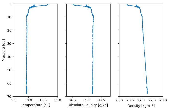
Plot vertical profile of temperature, salinity and density#
1.6 Describe what you can about the hydrographic structure from this plot.
# calculate salinity and density using the TEOS GSW package.

SP=gsw.SP_from_C(dat_hL1.COND[0,:],dat_hL1.TEMP,dat_hL1.PRES)
SA=gsw.SA_from_SP(SP,dat_hL1.PRES,-123,48)
CT =gsw.CT_from_t(SA,dat_hL1.TEMP,dat_hL1.PRES)
rho=gsw.rho(SA,CT,dat_hL1.PRES)
fig,ax=plt.subplots(1,3,figsize=(8,5),sharey=True)
ax[0].plot(CT,dat_hL1.PRES)
ax[0].set_ylim(70,0)
ax[0].set_xlim(9.5,11)
ax[0].set_ylabel('Pressure [db]')
ax[0].set_xlabel('Temperature [°C]')

ax[1].plot(SA,dat_hL1.PRES)
ax[1].set_xlim(34.3,35.8)
ax[1].set_xlabel('Absolute Salinity [g/kg]')

ax[2].plot(rho-1000,dat_hL1.PRES)
ax[2].set_xlim(26,28)
ax[2].set_xlabel('Density [kgm$^{-3}$]')
Text(0.5, 0, 'Density [kgm$^{-3}$]')
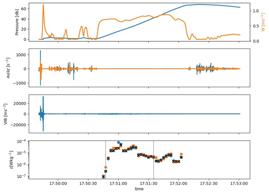
Plot time series#
Like before, below are time series of a) Pressure and Velocity through water, b) vertical shear, c) platform vibrations and d) turbulence dissipation rate.
1.7) Interpret what might be causing the enhanced vertical shear in b) with reference to the platofrms velocity through water.
1.8a) Describe the vertical profile of the dissipation rate of turbulence (where dissipation rate is high, where it is low) with reference to the distance from the surface and the temperature profile. Comment on differences to the previous profile in the Baltic Sea.
1.8b) Select two points, one with high dissipation rate and one with low dissipation rate and overlay vertical lines at these chosen points in subpanels d).
fig,ax=plt.subplots(4,1,figsize=(10,8),sharex=True)

ax[0].plot(dat_hL1.TIME,dat_hL1.PRES,lw=2)
ax[0].set_ylabel('Pressure [db]')

axa=ax[0].twinx()
axa.plot(dat_hL2.TIME,dat_hL2.PSPD_REL,c='tab:orange',lw=2)
axa.set_ylabel('W [ms$^{-1}$]',c='tab:orange')


ax[1].plot(dat_hL2.TIME,dat_hL2.SHEAR[0,:])
ax[1].plot(dat_hL2.TIME,dat_hL2.SHEAR[1,:])

ax[1].set_ylabel(r'$\partial u / \partial z$ [s$^{-1}$]')

ax[2].plot(dat_hL2.TIME,dat_hL2.VIB[0,:])
ax[2].set_ylabel(r'VIB [ms$^{-2}$]')


ax[3].scatter(dat_hL4.TIME,dat_hL4.EPSI[0,:],label=r'$\epsilon_1$')
ax[3].scatter(dat_hL4.TIME,dat_hL4.EPSI[1,:],label=r'$\epsilon_2$')
ax[3].scatter(dat_hL4.TIME,dat_hL4.EPSI_FINAL,c='k',marker='x',label=r'$\epsilon$')


### EDIT HERE, only dummies used
#identify two regions of dissipation (strong versus quiescent)
i= 20   # strong dissipation
j= 1   # weak dissipation

ax[3].axvline(pd.to_datetime(dat_hL4.TIME[i].values),c='grey',lw=1)
ax[3].axvline(pd.to_datetime(dat_hL4.TIME[j].values),c='grey',lw=1)

ax[3].set_yscale('log')
ax[3].set_ylabel(r'$\epsilon \mathrm{[W kg^{-1}]}$')
ax[3].set_xlabel('time')
Text(0.5, 0, 'time')
Create model Nasmyth Spectra for chosen dissipation rates in the data#
# print dissipation values for chosen spectra and create model nasmyth shear spectra

knas_strong = np.linspace(0,100,len(dat_hL3.KCYC[:,i]))
print(dat_hL4.EPSI_FINAL[i])
nasmyth_strong = Nasfunc(knas_strong,dat_hL4.EPSI_FINAL[i].values)

print(dat_hL4.EPSI_FINAL[j])
knas_weak = np.linspace(0,100,len(dat_hL3.KCYC[:,j]))
nasmyth_weak = Nasfunc(knas_weak,dat_hL4.EPSI_FINAL[j].values)
<xarray.DataArray 'EPSI_FINAL' ()> Size: 8B
array(4.216252e-06)
Attributes:
    standard_name:  specific_turbulent_kinetic_energy_dissipation_in_sea_water
    units:          W kg-1
    long_name:      dissipation rate of turbulent kinetic energy per unit mas...
<xarray.DataArray 'EPSI_FINAL' ()> Size: 8B
array(2.579372e-07)
Attributes:
    standard_name:  specific_turbulent_kinetic_energy_dissipation_in_sea_water
    units:          W kg-1
    long_name:      dissipation rate of turbulent kinetic energy per unit mas...
Dissipation estimates from shear spectra#
Look at the agreement between dissipation estimates from the two spectra. Generally, turbulence can be observed to within a factor of two.
1.9) Plot shear spectra at the two dissipation rates that you chose earlier. How does shear spectra relate to dissipation rates?
fig,ax=plt.subplots(1,2,figsize=(10,4))
fig.subplots_adjust(wspace=0.3)

## Dissipation plot

ax[0].scatter(dat_hL4.EPSI[0,:],dat_hL4.EPSI[1,:],marker='^',s=5)

ax[0].set_yscale('log')
ax[0].set_xscale('log')

# Define the range for the 1-to-1 and confidence interval lines
x_vals = np.logspace(-7,
                     -4, 100)

# Plot 1:1 line
ax[0].plot(x_vals, x_vals, 'k')

# Plot factor of 2 confidence intervals
ax[0].plot(x_vals, 2 * x_vals, 'k:')
ax[0].plot(x_vals, 0.5* x_vals, 'k:')

ax[0].set_ylim(1e-7,1e-4)
ax[0].set_xlim(1e-7,1e-4)

ax[0].set_xlabel(r'$\epsilon_1 \mathrm{[W kg^{-1}]}$')
ax[0].set_ylabel(r'$\epsilon_2 \mathrm{[W kg^{-1}]}$')


## Spectra

ax[1].plot(dat_hL3.KCYC[:,i],dat_hL3.SH_SPEC_CLEAN[0,:,i],c='tab:blue',lw=1,label=r'$\Psi_{1}$')
ax[1].plot(dat_hL3.KCYC[:,i],dat_hL3.SH_SPEC_CLEAN[1,:,i],c='tab:orange',lw=1,label=r'$\Psi_{2}$')
ax[1].plot(knas_strong,nasmyth_strong,c='grey',lw=1,label='Nasmyth Spectra')

ax[1].plot(dat_hL3.KCYC[:,j],dat_hL3.SH_SPEC_CLEAN[0,:,j],c='tab:blue',lw=1)
ax[1].plot(dat_hL3.KCYC[:,j],dat_hL3.SH_SPEC_CLEAN[1,:,j],c='tab:orange',lw=1)
ax[1].plot(knas_weak,nasmyth_weak,c='grey',lw=1)

ax[1].set_yscale('log')
ax[1].set_xscale('log')

ax[1].set_xlim(0.5,1e2)
ax[1].set_ylim(1e-6,1e-1)

ax[1].legend()

ax[1].set_xlabel(r'$k$ [cpm]')
ax[1].set_ylabel(r'$\Psi$ $[s^{-2}\mathrm{cpm}^{-1}]$')
Text(0, 0.5, '$\\Psi$ $[s^{-2}\\mathrm{cpm}^{-1}]$')
Part II#
Use observations of microstructure shear to understand turbulent processes in the ocean
Weddell Sea#
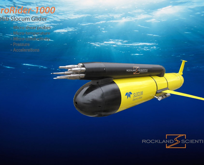
Fig. 25 A Rockland Scientific Microrider mounted on top of a Slocum glider.#
In this part, we will focus on a dataset collected by a Rocklands Scientific Microrider that was mounted on a Slocum glider and deployed in the seasonal sea-ice region of the Weddell Sea. Refer to [GFSN23] for context.
As in Part I, start by looking at the spectra and dissipation rates.
# First look at the global attributes
dat_a=xr.open_dataset('assignment/weddell_sea/DAT_190.nc', engine="h5netcdf",group="")
dat_a.attrs
{'platform_type': 'sub-surface glider',
 'comment': "Ocean turbulence data were collected using a Slocum electric glider as platform. Glider was deployed and recovered during the 2019-2020 SANAE South African Antarctic base resupply cruise on the RV SA Agulhas II. The MR operated continously on both dives and climbs from the surface to a depth of 500 m. The data from the MR include measurements from 2 shear probes, 2-axis piezo-accelerometers (vibration), an inclinometer (pitch and roll) and a pressure transducer. The processing of the data and the format of this data set follows the recommendations and guidelines of the SCOR Working Group 160, ATOMIX (https://wiki.uib.no/atomix), and the processing was done using the standard Matlab tools provided by Rockland Scientific. One NetCDF file per instrument's native file (typically one file per cast) is provided. Each netCDF file includes 4 groups: 4 levels of microstructure data in ATOMIX format. L1_converted : full-resolution data converted to physical units L2_cleaned : selected signals that are filtered and/or despiked before spectral analysis. Time stamp and length of the signals are same as L1. L3_spectra : wavenumber spectra from shear probes and vibration sensors L4_dissipation: dissipation estimates together with quality control parameters Spectral calculation and dissipation rate estimate details are given in the attributes and processing parameters. Spectra are obtained using 2-s fft length. Dissipation estimates are obtained over 12s segments, overlapping by 6s (50% overlap). Detailed data processing parameters and choices can be found in the attributes. Shear and vibration spectra, their complex cross-spectra, and the cleaned shear spectra using the Goodman method are provided. L4 includes estimates from both shear probes, using the cleaned spectra, as well as their average, together with quality control parameters. The figure of merit (FOM) and mean absolute deviation (MAD) relative to the Nasmyth model spectrum are used. Data quality flags for dissipation estimates are summarized in the attributes of the variable EPSI_FLAGS in the L4 group. A final dissipation estimate, EPSI_FINAL, failing the data quality control is reported as NaN; however, the individual dissipation estimates from each probe are accessible in the EPSI parameter.",
 'conventions': 'CF-1.6, ACDD-1.3, ATOMIX',
 'history': 'Version 1',
 'data_mode': 'D',
 'area': 'Seasonal Ice Zone, Weddell Sea, Southern Ocean',
 'geospatial_lat_min': np.float64(-60.09980633683413),
 'geospatial_lat_max': np.float64(-60.09980633683413),
 'geospatial_lon_min': np.float64(0.16348079499333565),
 'geospatial_lon_max': np.float64(0.16348079499333565),
 'geospatial_vertical_min': np.float64(0.0),
 'geospatial_vertical_max': np.float64(500.0),
 'geospatial_vertical_positive': 'down',
 'time_coverage_start': '2019-12-29T04:40:03Z',
 'time_coverage_end': '2019-12-29T05:29:38Z',
 'creator_name': 'Giddy, Isabelle',
 'creator_email': 'isabelle.giddy@gu.se',
 'creator_url': 'https://socco.org.za/',
 'institution': 'Southern Ocean Carbon-Climate Observatory, CSIR',
 'authors': 'Giddy, Isabelle, Fer, Ilker, and Nicholson, Sarah-Anne.;',
 'project_name': 'Contemporary and Future Drivers of CO2 and Heat in the Southern Ocean',
 'cruise': 'SANAE59',
 'vessel': 'RV SA Agulhas II, IMO vessel number 9577135',
 'principal_investigator': 'Nicholson, S-A.',
 'contact': 'snicholson@csir.co.za',
 'references': 'https://wiki.uib.no/atomix/; Lueck, R., I. Fer, C. E. Bluteau, M. Dengler, H. P., R. Inoue, A. LeBoyer, S.-A. Nicholson, K. Schulz, and C. Stevens (2024), Best practices recommendations for estimating dissipation rates from shear probes, Frontiers in Marine Science, 11, https://doi.org/10.3389/fmars.2024.1334327. Krahmann, Gerd (2023) GEOMAR FB1-PO Matlab Slocum glider processing toolbox. https://doi.org/10.3289/SW_4_2023. Goodman, L., Levine, E. R., and Lueck, R. G. (2006). On Measuring the Terms of the Turbulent Kinetic Energy Budget from an AUV, Journal of Atmospheric and Oceanic Technology, 23, 977\udce2\udc80\udc93990, https://doi.org/10.1175/JTECH1889.1, 2006. TN-028, https://rocklandscientific.com/support/knowledge-base/technical-notes/',
 'acknowledgements': 'This data set is made possible by the funding the the South African National Research Foundation (SANAP200324510487) and the Department of Science and Innovation.',
 'keywords': 'Southern Ocean Seasonal Ice Zone, glider, mixing, turbulence, dissipation rate, microstructure, shear probes',
 'source': 'sub-surface glider',
 'license': 'http://creativecommons.org/licenses/by/4.0/',
 'citation': 'later',
 'instrument': 'MicroRider-1000LP',
 'instrument_serial_number': np.float64(334.0),
 'instrument_sample_rate': np.float64(512.0),
 'instrument_sampling_mode': 'continuous',
 'profiling_direction': 'glide',
 'aoa': np.float64(3.0),
 'fname': '/Volumes/IssMacExtension/South_BLS/MR216/ROAMMIZ_2019/L0/P/DAT_190.P',
 'gradC_method': 'high_pass',
 'gradT_method': 'high_pass',
 'hotel_file': '/Volumes/IssMacExtension/South_BLS/MR216/ROAMMIZ_2019/L1/reprocess/HOTEL/Slocum_hotelfile_forODAS_wet2.mat',
 'speed_cutout': np.float64(0.02),
 'speed_tau': np.float64(3.0),
 'time_offset': np.float64(-4.0),
 'vehicle': 'slocum_glider',
 'temperature_source': 'Found within hotel file.',
 'speed_source': 'Hotel file',
 'fields_from_hotel': 'speed,W,depth,P,P_CTD,T_CTD,S_CTD,aoa,pitch,roll,fin,bb700,bb470,chla,lon,lat',
 'setupfilestr': '; 2021-10-08 16:17:49 patched configuration string\n; Standard configuration setup.cfg file for a MicroRider on a TWE Slocum glider.\n; Created by RSI, 2015-10-13\n; Any line that starts with a semicolon, ";", is a comment and is ignored by \n;  software. Likewise, everything to the right of a semicolon is ignored.\n;  Use this feature to leave notes and to indicate that you have made changes \n;  to this file. Indicate the date (YYYY-MM-DD), your name and a brief \n;  description of your changes.\n; MicroRiders are internally recording instruments.\n; Edited for Nicholson MR1000 SN334, 2019-09-27 by RSI AB\n; Edited pressure coefficients to zero at RSI by subtracting 0.84 from coeff. 0   2019-09-27\n; Sensors shear and temperature have nominal values input in the setup file.\n\n; The first section is the [root] section. It determines the data \n;  acquisition parameters. It does not need to be declared explicitly.\n\nrate        = 512    ; The sampling rate of fast channels\nprefix      = dat_   ; The base name of your data files. A 3-digit \n\t\t\t\t\t ;  file number is appended to this base name.\n\t\t\t\t\t ; The limit is 8 characters total for internally\n                     ;  recording instruments.\ndisk        = /data  ; The directory for the data files. Use /data only.\nrecsize     = 1      ; The size of a record in seconds\nno-fast     = 6      ; number of fast "columns" in the address matrix (see below).\nno-slow     = 2      ; number of slow "columns" in the address matrix.\n\n; -----------------\n;This section presents the address [matrix] of your instrument and \n;  automatically ends the [root] section above. The first columns are "slow"\n;  channels as defined by the "no-slow" parameter in the [root] section.\n;  The remainder are "fast" columns ("no-fast").\n[matrix]\nnum_rows=8\nrow01   =\t255\t0\t1\t2\t5\t7\t8\t9\t\t\nrow02   =\t32\t40\t1\t2\t5\t7\t8\t9\t\nrow03   =\t41\t42\t1\t2\t5\t7\t8\t9\t\nrow04   =\t4\t6\t1\t2\t5\t7\t8\t9\t\nrow05   =\t10\t11\t1\t2\t5\t7\t8\t9\t\nrow06   =\t12\t0\t1\t2\t5\t7\t8\t9\t\nrow07   =\t0\t0\t1\t2\t5\t7\t8\t9\t\nrow08   =\t0\t0\t1\t2\t5\t7\t8\t9\t\n\n; --------------------\n;This section identifies your instrument. Only the vehicle is important.\n[instrument_info]\nvehicle = slocum_glider ; up- and down-profiling\nmodel   = mr_1000       ; the actual model\nsn      = 334           ; the serial number of the instrument\n\n; --------------------\n; The next section is optional and can be expanded. Do not use the parameter "id = ".\n[cruise_info]\noperator    = Nicholson\nproject     = roammiz\nship        =\nleg         =\nglider      = \n\n; --------------------\n; Next come the [channel] sections. These are used to convert your data \n;  into physical units, and to save them into a mat-file. \n;  They also determine the name given to various signals \n;  in your data file. Please, stick to the convention of \n;  RSI because data visualization using the RSI Matlab Library of functions\n;  assumes particular names. However, data will be converted into physical\n;  units regardless of the name of the channels. If you change the names,\n;  then data visualization and further processing is your responsibility.\n;  A list of typical channel addresses (id) and their names and functions\n;  is at the end of this file.\n\n; Each channel section consists of a part that is unique to your instrument.\n;  It does not need to be changed. The second part is dependent on your \n;  sensors (shear probes, FP07 thermistors, etc.) and must be updated \n;  whenever you change a probe.\n\n; The ground reference channel.\n[channel]\nid      = 0   ; the channel address, 0 to 255.  Listed in the [matrix] section.\nname    = Gnd ; the name it will have in the mat-file.\ntype    = gnd ; the algorithm used to convert raw data into physical units.\ncoef0   = 0   ; the coefficients required for conversion. None in this case.\n\n; --------------\n; The piezo-vibration sensors\n[channel]\nid      = 1\nname    = Ax\ntype    = piezo\n\n[channel]\nid      = 2\nname    = Ay\ntype    = piezo\n\n; -----------------\n; The thermistor channels\n; without pre-emphasis\n[channel]\nid=4\nname=T1\ntype=therm\n; instrument dependent parameters\nadc_fs  = 4.096\nadc_bits= 16\na       =-7.5\nb       = 0.99822\nG       = 6.0\nE_B     = 0.68218\n; sensor dependent parameters. To be changed by user.\nSN      = T\nbeta_1  = 3143.55\nbeta_2  = 2.5e5\nT_0     = 289.301\ncal_date=\n; units = [C]\n\n; with pre-emphasis\n[channel]\nid          = 5\nname        = T1_dT1\ntype        = therm\n; instrument dependent parameter\ndiff_gain   = 0.930\n\n; without pre-emphasis\n[channel]\nid      = 6\nname    = T2\ntype    = therm\n; instrument dependent parameters\nadc_fs  = 4.096\nadc_bits= 16\na       =-9.3\nb       = 0.99821\nG       = 6.0\nE_B     = 0.68228\n; sensor dependent parameters. To be changed by user.\nSN      = T\nbeta_1  = 3143.55\nbeta_2  = 2.5e5\nT_0     = 289.301\ncal_date=\n; units = [C]\n\n; with pre-emphasis\n[channel]\nid          = 7\nname        = T2_dT2\ntype        = therm\ndiff_gain   = 0.926\n\n; -----------------\n; The shear probe channels\n[channel]\nid          = 8\nname        = sh1\ntype        = shear\n; instrument dependent parameters\nadc_fs      = 4.096\nadc_bits    = 16\ndiff_gain   = 0.936\n; sensor dependent parameters. To be changed by user.\nsens        = 0.0517\nSN          = M2076\ncal_date    =\n\n[channel]\nid          = 9\nname        = sh2\ntype        = shear\n; instrument dependent parameters\nadc_fs      = 4.096\nadc_bits    = 16\ndiff_gain   = 0.939\n; sensor dependent parameters. To be changed by user.\nsens        = 0.0753\nSN          = M2091\ncal_date    =\n\n; -----------------\n; The pressure transducer\n; without pre-emphasis\n[channel]\nid          = 10\nname        = P\ntype        = poly\n; instrument dependent parameters\ncoef0       = -4.87      ;offset reading to zero. -4.03(coef0) - 0.84(p.ch. reading)= -4.87\ncoef1       = 0.061704\ncoef2       = 3.3024e-8\ncal_date    = 2019-09-26\n;units       = [dBar]\n\n; with pre-emphasis\n[channel]\nid          = 11\nname        = P_dP\ntype        = poly\n; instrument dependent parameters\ndiff_gain   = 20.58\n\n; pressure transducer voltage\n[channel]\nid      = 12\nname    = PV\ntype    = poly\n; instrument dependent parameters\ncoef0   = 4.096\ncoef1   = 1.25e-4\n; units   = [V]\n\n; -----------------\n; Battery voltage or power supply voltage\n[channel]\nid          = 32\nname        = V_Bat\ntype        = voltage\n; instrument dependent parameters\nG           = 0.1\nadc_fs      = 4.096\nadc_bits    = 16\n; units       = [V]\n\n; -----------------\n; The ADIS precision inclinometer with built in thermometer\n[channel]\nid      = 40\nname    = Incl_Y\ntype    = inclxy\n; instrument dependent parameters\ncoef0   = 0\ncoef1   = 0.025\n; units   = [degree]\n\n[channel]\nid      = 41\nname    = Incl_X\ntype    = inclxy\n; instrument dependent parameters\ncoef0   = 0\ncoef1   = -0.025\n; units   = [degree]\n\n[channel]\nid      = 42\nname    = Incl_T\ntype    = inclt\n; instrument dependent parameters\ncoef0   = 624\ncoef1   =-0.47\n; units   = [C]\n\n; ------------------\n; This is a list of typical channels (addresses) and their signals\n; that are currently available for a MicroRider on a TWE Slocum glider.\n\n;  id     Name   - rate - Signal\n; -------------------------------------------------------------------\n;  0     Gnd     - slow - Reference ground\n;  1     Ax      - fast - horizontal acceleration in the direction of the pressure port or ON/OFF magnet\n;  2     Ay      - fast - horizontal acceleration orthogonal to the direction of the pressure port\n;  4     T1      - slow - Temperature from Thermistor 1 without pre-emphasis\n;  5     T1_dT1  - fast - Temperature from Thermistor 1 with pre-emphasis\n;  6     T2      - slow - Temperature from Thermistor 2 without pre-emphasis\n;  7     T2_dT2  - fast - Temperature from Thermistor 2 with pre-emphasis\n;  8     sh1     - fast - velocity derivative from shear probe 1\n;  9 \t sh2     - fast - velocity derivative from shear probe 2\n; 10     P       - slow - pressure signal without pre-emphasis\n; 11     P_dP    - slow - pressure signal with pre-emphasis\n; 12     PV      - slow - voltage on pressure transducer\n; 32     V_Bat   - slow - Battery or power supply voltage\n; 40     Incl_Y  - slow - Inclinometer, rotation around the y-axis\n; 41     Incl_X  - slow - Inclinometer, rotation around the x-axis\n; 42     Incl_T  - slow - Inclinometer, its temperature \n; 255    sp_char - slow - special Character that always returns 32752D or 7FF0H and \n;                         is used to test the integrity of communication.\n\n; End of setup configuration file.\n\n\n\n; ### Original Configuration String Below ###\n; ; Standard configuration setup.cfg file for a MicroRider on a TWE Slocum glider.\n; ; Created by RSI, 2015-10-13\n; ; Any line that starts with a semicolon, ";", is a comment and is ignored by \n; ;  software. Likewise, everything to the right of a semicolon is ignored.\n; ;  Use this feature to leave notes and to indicate that you have made changes \n; ;  to this file. Indicate the date (YYYY-MM-DD), your name and a brief \n; ;  description of your changes.\n; ; MicroRiders are internally recording instruments.\n; ; Edited for Nicholson MR1000 SN334, 2019-09-27 by RSI AB\n; ; Edited pressure coefficients to zero at RSI by subtracting 0.84 from coeff. 0   2019-09-27\n; ; Sensors shear and temperature have nominal values input in the setup file.\n; \n; ; The first section is the [root] section. It determines the data \n; ;  acquisition parameters. It does not need to be declared explicitly.\n; \n; rate        = 512    ; The sampling rate of fast channels\n; prefix      = dat_   ; The base name of your data files. A 3-digit \n; \t\t\t\t\t ;  file number is appended to this base name.\n; \t\t\t\t\t ; The limit is 8 characters total for internally\n;                      ;  recording instruments.\n; disk        = /data  ; The directory for the data files. Use /data only.\n; recsize     = 1      ; The size of a record in seconds\n; no-fast     = 6      ; number of fast "columns" in the address matrix (see below).\n; no-slow     = 2      ; number of slow "columns" in the address matrix.\n; \n; ; -----------------\n; ;This section presents the address [matrix] of your instrument and \n; ;  automatically ends the [root] section above. The first columns are "slow"\n; ;  channels as defined by the "no-slow" parameter in the [root] section.\n; ;  The remainder are "fast" columns ("no-fast").\n; [matrix]\n; num_rows=8\n; row01   =\t255\t0\t1\t2\t5\t7\t8\t9\t\t\n; row02   =\t32\t40\t1\t2\t5\t7\t8\t9\t\n; row03   =\t41\t42\t1\t2\t5\t7\t8\t9\t\n; row04   =\t4\t6\t1\t2\t5\t7\t8\t9\t\n; row05   =\t10\t11\t1\t2\t5\t7\t8\t9\t\n; row06   =\t12\t0\t1\t2\t5\t7\t8\t9\t\n; row07   =\t0\t0\t1\t2\t5\t7\t8\t9\t\n; row08   =\t0\t0\t1\t2\t5\t7\t8\t9\t\n; \n; ; --------------------\n; ;This section identifies your instrument. Only the vehicle is important.\n; [instrument_info]\n; vehicle = slocum_glider ; up- and down-profiling\n; model   = mr_1000       ; the actual model\n; sn      = 334           ; the serial number of the instrument\n; \n; ; --------------------\n; ; The next section is optional and can be expanded. Do not use the parameter "id = ".\n; [cruise_info]\n; operator    = Nicholson\n; project     = \n; ship        =\n; leg         =\n; glider      =\n; \n; ; --------------------\n; ; Next come the [channel] sections. These are used to convert your data \n; ;  into physical units, and to save them into a mat-file. \n; ;  They also determine the name given to various signals \n; ;  in your data file. Please, stick to the convention of \n; ;  RSI because data visualization using the RSI Matlab Library of functions\n; ;  assumes particular names. However, data will be converted into physical\n; ;  units regardless of the name of the channels. If you change the names,\n; ;  then data visualization and further processing is your responsibility.\n; ;  A list of typical channel addresses (id) and their names and functions\n; ;  is at the end of this file.\n; \n; ; Each channel section consists of a part that is unique to your instrument.\n; ;  It does not need to be changed. The second part is dependent on your \n; ;  sensors (shear probes, FP07 thermistors, etc.) and must be updated \n; ;  whenever you change a probe.\n; \n; ; The ground reference channel.\n; [channel]\n; id      = 0   ; the channel address, 0 to 255.  Listed in the [matrix] section.\n; name    = Gnd ; the name it will have in the mat-file.\n; type    = gnd ; the algorithm used to convert raw data into physical units.\n; coef0   = 0   ; the coefficients required for conversion. None in this case.\n; \n; ; --------------\n; ; The piezo-vibration sensors\n; [channel]\n; id      = 1\n; name    = Ax\n; type    = piezo\n; \n; [channel]\n; id      = 2\n; name    = Ay\n; type    = piezo\n; \n; ; -----------------\n; ; The thermistor channels\n; ; without pre-emphasis\n; [channel]\n; id=4\n; name=T1\n; type=therm\n; ; instrument dependent parameters\n; adc_fs  = 4.096\n; adc_bits= 16\n; a       =-7.5\n; b       = 0.99822\n; G       = 6.0\n; E_B     = 0.68218\n; ; sensor dependent parameters. To be changed by user.\n; SN      = T\n; beta_1  = 3143.55\n; beta_2  = 2.5e5\n; T_0     = 289.301\n; cal_date=\n; ; units = [C]\n; \n; ; with pre-emphasis\n; [channel]\n; id          = 5\n; name        = T1_dT1\n; type        = therm\n; ; instrument dependent parameter\n; diff_gain   = 0.930\n; \n; ; without pre-emphasis\n; [channel]\n; id      = 6\n; name    = T2\n; type    = therm\n; ; instrument dependent parameters\n; adc_fs  = 4.096\n; adc_bits= 16\n; a       =-9.3\n; b       = 0.99821\n; G       = 6.0\n; E_B     = 0.68228\n; ; sensor dependent parameters. To be changed by user.\n; SN      = T\n; beta_1  = 3143.55\n; beta_2  = 2.5e5\n; T_0     = 289.301\n; cal_date=\n; ; units = [C]\n; \n; ; with pre-emphasis\n; [channel]\n; id          = 7\n; name        = T2_dT2\n; type        = therm\n; diff_gain   = 0.926\n; \n; ; -----------------\n; ; The shear probe channels\n; [channel]\n; id          = 8\n; name        = sh1\n; type        = shear\n; ; instrument dependent parameters\n; adc_fs      = 4.096\n; adc_bits    = 16\n; diff_gain   = 0.936\n; ; sensor dependent parameters. To be changed by user.\n; sens        = 0.0700\n; SN          = M\n; cal_date    =\n; \n; [channel]\n; id          = 9\n; name        = sh2\n; type        = shear\n; ; instrument dependent parameters\n; adc_fs      = 4.096\n; adc_bits    = 16\n; diff_gain   = 0.939\n; ; sensor dependent parameters. To be changed by user.\n; sens        = 0.0700\n; SN          = M\n; cal_date    =\n; \n; ; -----------------\n; ; The pressure transducer\n; ; without pre-emphasis\n; [channel]\n; id          = 10\n; name        = P\n; type        = poly\n; ; instrument dependent parameters\n; coef0       = -4.87      ;offset reading to zero. -4.03(coef0) - 0.84(p.ch. reading)= -4.87\n; coef1       = 0.061704\n; coef2       = 3.3024e-8\n; cal_date    = 2019-09-26\n; ;units       = [dBar]\n; \n; ; with pre-emphasis\n; [channel]\n; id          = 11\n; name        = P_dP\n; type        = poly\n; ; instrument dependent parameters\n; diff_gain   = 20.58\n; \n; ; pressure transducer voltage\n; [channel]\n; id      = 12\n; name    = PV\n; type    = poly\n; ; instrument dependent parameters\n; coef0   = 4.096\n; coef1   = 1.25e-4\n; ; units   = [V]\n; \n; ; -----------------\n; ; Battery voltage or power supply voltage\n; [channel]\n; id          = 32\n; name        = V_Bat\n; type        = voltage\n; ; instrument dependent parameters\n; G           = 0.1\n; adc_fs      = 4.096\n; adc_bits    = 16\n; ; units       = [V]\n; \n; ; -----------------\n; ; The ADIS precision inclinometer with built in thermometer\n; [channel]\n; id      = 40\n; name    = Incl_Y\n; type    = inclxy\n; ; instrument dependent parameters\n; coef0   = 0\n; coef1   = 0.025\n; ; units   = [degree]\n; \n; [channel]\n; id      = 41\n; name    = Incl_X\n; type    = inclxy\n; ; instrument dependent parameters\n; coef0   = 0\n; coef1   = -0.025\n; ; units   = [degree]\n; \n; [channel]\n; id      = 42\n; name    = Incl_T\n; type    = inclt\n; ; instrument dependent parameters\n; coef0   = 624\n; coef1   =-0.47\n; ; units   = [C]\n; \n; ; ------------------\n; ; This is a list of typical channels (addresses) and their signals\n; ; that are currently available for a MicroRider on a TWE Slocum glider.\n; \n; ;  id     Name   - rate - Signal\n; ; -------------------------------------------------------------------\n; ;  0     Gnd     - slow - Reference ground\n; ;  1     Ax      - fast - horizontal acceleration in the direction of the pressure port or ON/OFF magnet\n; ;  2     Ay      - fast - horizontal acceleration orthogonal to the direction of the pressure port\n; ;  4     T1      - slow - Temperature from Thermistor 1 without pre-emphasis\n; ;  5     T1_dT1  - fast - Temperature from Thermistor 1 with pre-emphasis\n; ;  6     T2      - slow - Temperature from Thermistor 2 without pre-emphasis\n; ;  7     T2_dT2  - fast - Temperature from Thermistor 2 with pre-emphasis\n; ;  8     sh1     - fast - velocity derivative from shear probe 1\n; ;  9 \t sh2     - fast - velocity derivative from shear probe 2\n; ; 10     P       - slow - pressure signal without pre-emphasis\n; ; 11     P_dP    - slow - pressure signal with pre-emphasis\n; ; 12     PV      - slow - voltage on pressure transducer\n; ; 32     V_Bat   - slow - Battery or power supply voltage\n; ; 40     Incl_Y  - slow - Inclinometer, rotation around the y-axis\n; ; 41     Incl_X  - slow - Inclinometer, rotation around the x-axis\n; ; 42     Incl_T  - slow - Inclinometer, its temperature \n; ; 255    sp_char - slow - special Character that always returns 32752D or 7FF0H and \n; ;                         is used to test the integrity of communication.\n; \n; ; End of setup configuration file.\n; \n; ',
 'date': '29-Dec-2019 04:40:03',
 'time_reference_year': np.float64(2020.0),
 'profile_dir': 'glide',
 'fs_slow': np.float64(64.00409375),
 'fs_fast': np.float64(512.03275),
 'fft_length_sec': np.float64(2.0),
 'diss_length_sec': np.float64(12.0),
 'overlap_sec': np.float64(6.0),
 'fft_length': np.float64(1024.0),
 'diss_length': np.float64(6144.0),
 'overlap': np.float64(3072.0),
 'goodman': np.float32(1.0),
 'fit_order': np.float64(3.0),
 'f_AA': np.float64(98.0),
 'profile_min_W': np.float64(0.15),
 'profile_min_duration': np.float64(30.0),
 'profile_min_P': np.float64(1.0),
 'HP_cut': np.float64(0.25),
 'despike_sh': array([8.  , 0.3 , 0.04]),
 'despike_A': array([8.  , 0.3 , 0.04]),
 'despike_shear_fraction_limit': np.float64(0.2),
 'FOM_limit': np.float64(1.15),
 'diss_ratio_limit': np.float64(2.772),
 'despike_shear_iterations_limit': np.float64(11.0),
 'min_pitch_threshold': np.float64(5.0),
 'vibrations_removed_indices': array([ 103975.,  103976.,  103977., ..., 1484968., 1484969., 1484970.],
       shape=(55796,)),
 'vibrations_removed_percent': np.float64(3.661846858198925),
 'spectral_model': 'Lueck',
 'refine_section': np.float64(1.0),
 'variance_resolved_limit': np.float64(0.5),
 'fit_2_isr': np.float64(1.5e-05),
 'f_limit': np.float64(inf),
 'num_vibration_goodman': np.float64(2.0),
 'num_fft_segments': np.float64(11.0),
 'spectrum_std': np.float64(0.4757301730292029),
 'PMAX': np.float64(510.10317381282397),
 'LON': np.float64(0.16348079499333565),
 'LAT': np.float64(-60.09980633683413),
 'creation_time': '2025-02-05T14:02:40Z',
 'date_update': '2025-02-05T14:02:40Z',
 'date_created': '2025-02-05',
 'title': 'Dissipation measurements from a Slocum Glider in the Southern Ocean during austral summer 2017, 2018 and 2019',
 'summary': 'This dataset includes data from 3 missions in the Southern Ocean between 2017 and 2020. This data file is for the mission in the Seasonal Ice Zone between 2019 and 2020. Ocean microstructure data were collected using a turbulence package mounted on a Slocum and deployed from RV SA Agulhas II in the North Eastern Weddell Sea, [60S; 0E], from December 2019 to February 2020. Observations conducted by the Southern Ocean Carbon-Climate Observatory, Smart Places, CSIR, for the project "Contemporary and Future Drivers of CO2 and Heat in the Southern Ocean" funded by NRF-SANAP (SANAP200324510487) and in collaboration with Polar Gliders, University of Gothenburg (Project "Robotic Observations and Modelling of the Marginal Ice Zone" funded by the Wallenberg Academy Fellowship (WAF 2015.0186). Turbulence data were collected using a Rockland Scientific MicroRider mounted on the SLOCUM. Microshear was measured using two airfoil shear probes oriented orthogonally to each other. The measurements are from 47 days of dive and climb profiles. The glider profiled to 1000 m, but the MicroRider only recorded to 500 m. Dissipation rate was measured using two airfoil shear probes. The dissipation dataset is processed and prepared following the SCOR Working Group ATOMIX guidelines and convention (Lueck et al., 2024). The glider data are processed using the GEOMAR Matlab Slocum glider processing toolbox (Krahmann, 2023). One NetCDF(NC) file per instrument\'s native file (typically one file per cast) is provided. Each provided NC file includes four hierarchical groups. Each consists of a continuous time series of full-resolution data converted into physical units; the cleaned time series used for spectral analysis, wavenumber spectra, and the dissipation rate estimates. Because each file includes full-resolution data at two levels and full-resolution spectra in the third group, the grouped NC files are large in size and may be unpractical to download and merge. For users only interested in the dissipation and the glider flight metrics and CTD profiles (in the hotel file), we also provide two separate NC files with all sections from the L4_dissipation and the hotel file collated into one file each. Further details are provided in the comments.'}
dat_wL1=xr.open_dataset('assignment/weddell_sea/DAT_190.nc', engine="h5netcdf",group="L1_converted")
dat_wL2=xr.open_dataset('assignment/weddell_sea/DAT_190.nc', engine="h5netcdf",group="L2_cleaned")
dat_wL3=xr.open_dataset('assignment/weddell_sea/DAT_190.nc', engine="h5netcdf",group="L3_spectra")
dat_wL4=xr.open_dataset('assignment/weddell_sea/DAT_190.nc', engine="h5netcdf",group="L4_dissipation")
Plot vertical profile of temperature, salinity, density and vertical stratification#
2.1 Describe what you can about the hydrographic structure from this plot.
# calculate density and stratification
rho=gsw.rho(dat_wL1.SALT,dat_wL1.TEMP_CTD,dat_wL1.PRES_SLOW)

rho_sorted =np.sort(rho)

# Compute brunt-vaisala frequency
g=9.8
p0=1025
# n2 = g/p0*(np.diff(rho_sorted)/np.diff(low_res_ctd.z))
drho_dz = np.gradient(rho_sorted, dat_wL1.PRES_SLOW)
n2 = g/p0*drho_dz

def smooth(x, window_len=5):
    return np.convolve(x, np.ones(window_len)/window_len, mode='same')

n2_smooth = smooth(n2, window_len=1000)
/Users/xnunei/miniconda3/envs/jb/lib/python3.13/site-packages/numpy/lib/_function_base_impl.py:1290: RuntimeWarning: divide by zero encountered in divide
  a = -(dx2)/(dx1 * (dx1 + dx2))
/Users/xnunei/miniconda3/envs/jb/lib/python3.13/site-packages/numpy/lib/_function_base_impl.py:1290: RuntimeWarning: invalid value encountered in divide
  a = -(dx2)/(dx1 * (dx1 + dx2))
/Users/xnunei/miniconda3/envs/jb/lib/python3.13/site-packages/numpy/lib/_function_base_impl.py:1291: RuntimeWarning: divide by zero encountered in divide
  b = (dx2 - dx1) / (dx1 * dx2)
/Users/xnunei/miniconda3/envs/jb/lib/python3.13/site-packages/numpy/lib/_function_base_impl.py:1291: RuntimeWarning: invalid value encountered in divide
  b = (dx2 - dx1) / (dx1 * dx2)
/Users/xnunei/miniconda3/envs/jb/lib/python3.13/site-packages/numpy/lib/_function_base_impl.py:1292: RuntimeWarning: divide by zero encountered in divide
  c = dx1 / (dx2 * (dx1 + dx2))
/Users/xnunei/miniconda3/envs/jb/lib/python3.13/site-packages/numpy/lib/_function_base_impl.py:1292: RuntimeWarning: invalid value encountered in divide
  c = dx1 / (dx2 * (dx1 + dx2))
/Users/xnunei/miniconda3/envs/jb/lib/python3.13/site-packages/numpy/lib/_function_base_impl.py:1298: RuntimeWarning: invalid value encountered in add
  out[tuple(slice1)] = a * f[tuple(slice2)] + b * f[tuple(slice3)] + c * f[tuple(slice4)]
/Users/xnunei/miniconda3/envs/jb/lib/python3.13/site-packages/numpy/lib/_function_base_impl.py:1307: RuntimeWarning: divide by zero encountered in scalar divide
  out[tuple(slice1)] = (f[tuple(slice2)] - f[tuple(slice3)]) / dx_0
/Users/xnunei/miniconda3/envs/jb/lib/python3.13/site-packages/numpy/lib/_function_base_impl.py:1314: RuntimeWarning: invalid value encountered in scalar divide
  out[tuple(slice1)] = (f[tuple(slice2)] - f[tuple(slice3)]) / dx_n
fig,ax=plt.subplots(1,4,figsize=(10,5),sharey=True)
ax[0].plot(dat_wL1.TEMP_CTD,dat_wL1.PRES_SLOW)
ax[0].set_ylim(150,0)
# ax[0].set_xlim(9.5,11)
ax[0].set_ylabel('Pressure [db]')
ax[0].set_xlabel('Temperature [°C]')

ax[1].plot(dat_wL1.SALT,dat_wL1.PRES_SLOW)
# ax[1].set_xlim(34.3,35.8)
ax[1].set_xlabel('Absolute Salinity [g/kg]')

ax[2].plot(rho-1000,dat_wL1.PRES_SLOW)
ax[2].set_xlim(27,28.5)
ax[2].set_xlabel('Density [kgm$^{-3}$]')


ax[3].plot(np.abs(n2),dat_wL1.PRES_SLOW[:])
ax[3].plot(np.abs(n2_smooth),dat_wL1.PRES_SLOW[:],c='k')

ax[3].set_xlim(1e-5,1e-3)
ax[3].set_xlabel('N$^2$ [s$^{-2}$]')
ax[3].set_xscale('log')
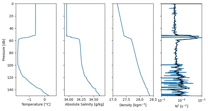
Plot time series#
Below are time series of a) Pressure and Velocity through water, b) vertical shear, c) platform vibrations and d) turbulence dissipation rate.
2.2a) Describe the vertical profile of the dissipation rate of turbulence (where dissipation rate is high, where it is low) with reference to the distance from the surface and the temperature profile.
2.2b) Select two points, one with high dissipation rate and one with low dissipation rate and overlay vertical lines at these chosen points in subpanels d).
fig,ax=plt.subplots(4,1,figsize=(10,8),sharex=True)

ax[0].plot(dat_wL1.TIME,dat_wL1.PRES,lw=2)
ax[0].set_ylabel('Pressure [db]')

axa=ax[0].twinx()
axa.plot(dat_wL2.TIME,dat_wL2.PSPD_REL,c='tab:orange',lw=2)
axa.set_ylabel('W [ms$^{-1}$]',c='tab:orange')


ax[1].plot(dat_wL2.TIME,dat_wL2.SHEAR[0,:])
ax[1].plot(dat_wL2.TIME,dat_wL2.SHEAR[1,:])

ax[1].set_ylabel(r'$\partial u / \partial z$ [s$^{-1}$]')

ax[2].plot(dat_wL2.TIME,dat_wL2.VIB[0,:])
ax[2].set_ylabel(r'VIB [ms$^{-2}$]')


ax[3].scatter(dat_wL4.TIME,dat_wL4.EPSI[0,:],label=r'$\epsilon_1$')
ax[3].scatter(dat_wL4.TIME,dat_wL4.EPSI[1,:],label=r'$\epsilon_2$')
ax[3].scatter(dat_wL4.TIME,dat_wL4.EPSI_FINAL,c='k',marker='x',label=r'$\epsilon$')

### EDIT HERE, only dummies used
# identify two regions of dissipation (strong versus quiescent)
i= 6   # strong dissipation
j= 90  # weak dissipation

ax[3].axvline(pd.to_datetime(dat_wL4.TIME[i].values),c='grey',lw=1)
ax[3].axvline(pd.to_datetime(dat_wL4.TIME[j].values),c='grey',lw=1)

ax[3].set_yscale('log')
ax[3].set_ylabel(r'$\epsilon \mathrm{[W kg^{-1}]}$')
ax[3].set_xlabel('time')
Text(0.5, 0, 'time')
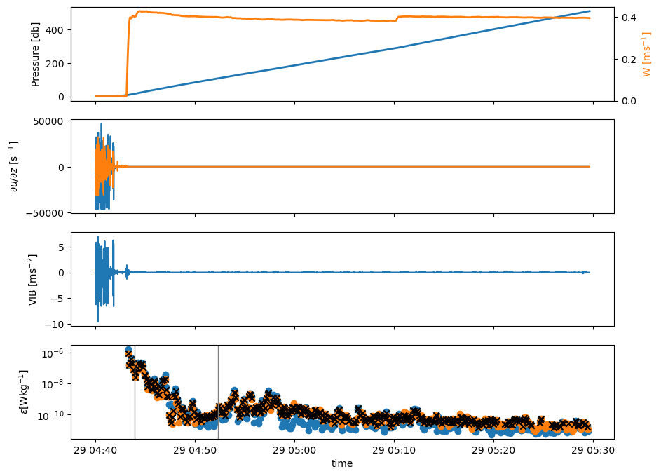
Create model Nasmyth Spectra for chosen dissipation rates in the data#
# print dissipation values for chosen spectra and create model nasmyth shear spectra

knas_strong = np.linspace(0,100,len(dat_wL3.KCYC[:,i]))
print(dat_wL4.EPSI_FINAL[i])
nasmyth_strong = Nasfunc(knas_strong,dat_wL4.EPSI_FINAL[i].values)

print(dat_wL4.EPSI_FINAL[j])
knas_weak = np.linspace(0,100,len(dat_wL3.KCYC[:,j]))
nasmyth_weak = Nasfunc(knas_weak,dat_wL4.EPSI_FINAL[j].values)
<xarray.DataArray 'EPSI_FINAL' ()> Size: 8B
array(4.929667e-08)
Attributes:
    standard_name:  specific_turbulent_kinetic_energy_dissipation_in_sea_water
    units:          W kg-1
    long_name:      dissipation rate of turbulent kinetic energy per unit mas...
<xarray.DataArray 'EPSI_FINAL' ()> Size: 8B
array(2.270163e-10)
Attributes:
    standard_name:  specific_turbulent_kinetic_energy_dissipation_in_sea_water
    units:          W kg-1
    long_name:      dissipation rate of turbulent kinetic energy per unit mas...
Dissipation estimates from shear spectra#
Look at the agreement between dissipation estimates from the two spectra. Generally, turbulence can be observed to within a factor of two.
2.3) Look at the dissipation estimates from tho probes. At which dissipation rate might you expect to be less condident about the results?
2.4) Plot shear spectra at the two dissipation rates that you chose earlier. How does shear spectra relate to dissipation rates?
fig,ax=plt.subplots(1,2,figsize=(10,4))
fig.subplots_adjust(wspace=0.3)

## Dissipation plot

ax[0].scatter(dat_wL4.EPSI[0,:],dat_wL4.EPSI[1,:],marker='^',s=5)

ax[0].set_yscale('log')
ax[0].set_xscale('log')

# Define the range for the 1-to-1 and confidence interval lines
x_vals = np.logspace(-11,
                     -5, 100)

# Plot 1:1 line
ax[0].plot(x_vals, x_vals, 'k')

# Plot factor of 2 confidence intervals
ax[0].plot(x_vals, 2 * x_vals, 'k:')
ax[0].plot(x_vals, 0.5* x_vals, 'k:')

ax[0].set_ylim(1e-11,1e-5)
ax[0].set_xlim(1e-11,1e-5)

ax[0].set_xlabel(r'$\epsilon_1 \mathrm{[W kg^{-1}]}$')
ax[0].set_ylabel(r'$\epsilon_2 \mathrm{[W kg^{-1}]}$')


## Spectra

ax[1].plot(dat_wL3.KCYC[:,i],dat_wL3.SH_SPEC_CLEAN[0,:,i],c='tab:blue',lw=1,label=r'$\Psi_{1}$')
ax[1].plot(dat_wL3.KCYC[:,i],dat_wL3.SH_SPEC_CLEAN[1,:,i],c='tab:orange',lw=1,label=r'$\Psi_{2}$')
ax[1].plot(knas_strong,nasmyth_strong,c='grey',lw=1,label='Nasmyth Spectra')

ax[1].plot(dat_wL3.KCYC[:,j],dat_wL3.SH_SPEC_CLEAN[0,:,j],c='tab:blue',lw=1)
ax[1].plot(dat_wL3.KCYC[:,j],dat_wL3.SH_SPEC_CLEAN[1,:,j],c='tab:orange',lw=1)
ax[1].plot(knas_weak,nasmyth_weak,c='grey',lw=1)

ax[1].set_yscale('log')
ax[1].set_xscale('log')

ax[1].set_xlim(0.5,1e2)
ax[1].set_ylim(1e-10,1e-1)

ax[1].legend()

ax[1].set_xlabel(r'$k$ [cpm]')
ax[1].set_ylabel(r'$\Psi$ $[s^{-2}\mathrm{cpm}^{-1}]$')
Text(0, 0.5, '$\\Psi$ $[s^{-2}\\mathrm{cpm}^{-1}]$')
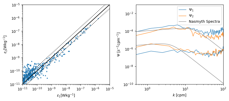
Compute the vertical turbulent heat flux#
Using the Eddy Diffusivity, \(Kz\) and following Osborn (1960), calculate the vertical turbulent heat flux.
Assuming the Osborn model for \(Kz\):
Note that because the Osborn model for eddy diffusivity is calculated as a function of \(N^2\), it will not be valid in conditions of very small \(N^2\). Where might this occur?
Heat flux, \(F_h\), can be approximated as:
2.5) What is the range of Eddy diffusivity? Is this comparable to expected values in the ocean?
2.6) Where is heat flux the strongest? What are possible explanations for the distribution of heat flux in this profile?
#interporate salinity to dissipation spectra
ds_interp = dat_wL1.SALT.interp(
    TIME_SLOW=dat_wL4.TIME
)

SA=ds_interp

# calculate density and stratification
rho=gsw.rho(SA,dat_wL4.TEMP,dat_wL4.PRES)

rho_sorted =np.sort(rho)

# Compute brunt-vaisala frequency
g=9.8
p0=1025
# n2 = g/p0*(np.diff(rho_sorted)/np.diff(low_res_ctd.z))
drho_dz = np.gradient(rho_sorted, dat_wL4.PRES)
n2 = g/p0*drho_dz
# Eddy diffusivity, k=0.2 epsilon/N2
# Osborn Model

Kz= 0.2*dat_wL4.EPSI_FINAL/np.abs(n2)
fig,ax=plt.subplots(1,5,figsize=(15,5),sharey=True)

rho0=1000
cp=4000

ax[0].plot(dat_wL4.EPSI_FINAL,dat_wL4.PRES)
ax[0].set_xscale('log')

ax[1].plot(Kz,dat_wL4.PRES)
ax[1].set_xscale('log')
ax[2].plot(dat_wL4.TEMP,dat_wL4.PRES)
ax[3].plot((np.gradient(dat_wL4.TEMP)/np.gradient(dat_wL4.PRES)),dat_wL4.PRES)
ax[4].plot(rho0*cp*Kz*(np.gradient(dat_wL4.TEMP)/np.gradient(dat_wL4.PRES)),dat_wL4.PRES)
ax[4].set_xlim(-5,5)
ax[3].set_ylim(180,0)

ax[0].set_ylabel('Depth  (m)')
ax[0].set_xlabel('$\epsilon \ (m^3s^{-2})$')
ax[1].set_xlabel('$K_z \ (m^2s^{-1})$')
ax[2].set_xlabel('Temperature  (°C)')
ax[3].set_xlabel(r'$\frac{dT}{dz}$  (°C m$^{-1}$)')
ax[4].set_xlabel('F$_h$  (W$m^{-2})$')
<>:18: SyntaxWarning: invalid escape sequence '\e'
<>:19: SyntaxWarning: invalid escape sequence '\ '
<>:18: SyntaxWarning: invalid escape sequence '\e'
<>:19: SyntaxWarning: invalid escape sequence '\ '
/var/folders/1q/qmm9yg_90xl7f60v6q7wn2fr0000gn/T/ipykernel_51571/2509822319.py:18: SyntaxWarning: invalid escape sequence '\e'
  ax[0].set_xlabel('$\epsilon \ (m^3s^{-2})$')
/var/folders/1q/qmm9yg_90xl7f60v6q7wn2fr0000gn/T/ipykernel_51571/2509822319.py:19: SyntaxWarning: invalid escape sequence '\ '
  ax[1].set_xlabel('$K_z \ (m^2s^{-1})$')
Text(0.5, 0, 'F$_h$ (W$m^{-2})$')
Compare the law-of-the-wall model for turbulent dissipation in a boundary layer with the observations#
Law of the wall:
2.7) What are the main assumptions of law-of-the-wall?
2.8) Up to what depth does law-of-the-wall agree with observations?
2.9) Given \(B_0 = 1 \times 10^{-8} \ m^3 s^{-2}\), compute the Monin-Obukhov length scale and make a statement about the forcing conditions experienced while this profile was taken.
\(z/L_{MO}<0.3\) , wind driven shear production
\(z/L_{MO}>1\) , buoyancy dominated (production or consumption)
# example
z=5
ustar=0.01
B=1e-8
L_MO=(ustar**3/(0.4*1e-8))
z/(ustar**3/(0.4*1e-8)) #z/L_MO less than 0.3, therefore at 5m the turbulence produciton is wind driven and L.O.W should apply
0.019999999999999997
# model profile
z=np.arange(0,80,1)
k=0.4
ustar=0.01
eps_low=ustar**3/(k*z)
eps_low_2x=eps_low*2
eps_low_2s=eps_low*0.5
/var/folders/1q/qmm9yg_90xl7f60v6q7wn2fr0000gn/T/ipykernel_51571/2175224984.py:5: RuntimeWarning: divide by zero encountered in divide
  eps_low=ustar**3/(k*z)
plt.figure()

plt.plot(eps_low,z,c='k',label='law-of-the-wall')
plt.plot(eps_low_2x,z,c='grey',ls='--')
plt.plot(eps_low_2s,z,c='grey',ls='--')


plt.plot(dat_wL4.EPSI_FINAL,dat_wL4.PRES,label='obs')
plt.xscale('log')
plt.ylim(80,0)
plt.ylabel('z [m]')
plt.xlabel('$\epsilon$ [W kg$^{-1}$]')
plt.legend()
<>:12: SyntaxWarning: invalid escape sequence '\e'
<>:12: SyntaxWarning: invalid escape sequence '\e'
/var/folders/1q/qmm9yg_90xl7f60v6q7wn2fr0000gn/T/ipykernel_51571/2234889368.py:12: SyntaxWarning: invalid escape sequence '\e'
  plt.xlabel('$\epsilon$ [W kg$^{-1}$]')
<matplotlib.legend.Legend at 0x1698cbed0>